20.5 Generalised symmetric merge
Note the set theoretic laws
(A⋃B)\C = (A\C) ⋃ (B\C)
A\(B⋂C) = (A\B) ⋃ (A\C)
In this section we generalise the merge operator ⊕ so it no longer assumes that the operations being merged are contextually serialised.
Let operations O1, O2 satisfy
vin(O1) ≤ v and vin(O2) ≤ v, where v = vout(O1) ↓ vout(O2).
Then we define:
O1 ⊕ O2 = ∑[ vin(O1)↓vin(O2), vout(O1)↑vout(O2) )
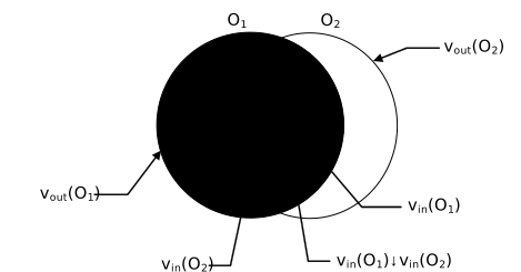
Let v = vout(O1) ↓ vout(O2). The condition implies vin(O1) ≤ v and vin(O2) ≤ v which in turn implies that it is possible to factorise both O1 and O2 with respect to v. Informally we say that O1,O2 have sufficient history.
Ignoring differences between vin(O1) and vin(O2), we could say that the merge of O1,O2 entails a dualIT between Rf(O1,v) and Rf(O2,v).
To simplify the control algorithm we regard the merge and factorisation operators as more fundamental than IT or ET!
Asymmetric merge
In this section we define a generalised asymmetric merge operator ⊕R.
Let operations O1, O2 satisfy:
vin(O1) ≤ v and vin(O2) ≤ v, where v = vout(O1) ↓ vout(O2).
Then:
O1 ⊕R O2 = ∑[ vin(O1), vout(O1)↑vout(O2))
Conceptually O1 ⊕R O2 is obtained by starting with O1 and merging in all the atomic operations that are in vout(O2) \ vout(O1).
It is not generally the case that Ψ(O1 ⊕R O2) = Ψ(O1) ⋃ Ψ(O2), because vin(O1 ⊕R O2) = vin(O1). This lack of symmetry in the definition means we don't generally expect O1 ⊕R O2 = O2 ⊕R O1 unless vin(O1) = vin(O2).
The condition vin(O1) ≤ v and vin(O2) ≤ v implies that it is possible to factorise both O1 and O2 with respect to v. Informally it means that O1,O2 each have sufficient history.
As for the symmetric merge, Rf(O1,v) || Rf(O2,v).
However in practice it doesn't make sense for the implementation to treat ⊕C and IT as independent operators, because merging implicitly involves dual IT, so it is better for the implementation to implement IT and merge as a single operator ⊕R. Furthermore the implementation should return the transformed O2, or else allow for O2 to be executed as part of the merge.
Using a single primitive merge operator
Consider that we avoid needing to treat database states within our mathematical model by thinking of a state as nothing more than the result of all the operations that created that state. Then if operations converge under merging it necessarily follows that database states do as well.
Furthermore let's pretend that operations happen to carry all the information required to be applied from the initial state. In other words an operation is identified with an entire history buffer and therefore is uniquely specified for a given output vector time. At this level of abstraction the execution context of the operation is irrelevant. This means that states and operations are really one and the same! We have in effect dropped the whole idea that operations represent deltas.
The point of this is to reduce the system to a single primitive operator (denoted by ⊕)that merges any two given operations (or states or history buffers if you prefer).
Let Ohb represent a site's entire history buffer. Ohb can also be regarded as an operation or a state. The control algorithm is very simple:
Note that there is no need to separately apply an operation because the database state is identified directly with Ohb.
The properties required of this operator are simply:
- O1 ⊕ O2 = O2 ⊕ O1
- (O1 ⊕ O2) ⊕ O3 = O1 ⊕ (O2 ⊕ O3)
Associativity and commutativity are sufficient to ensure all sites converge at quiescence. This can be compared to TP1 and TP2 properties for IT which is comparatively complex, particularly in light of the rather complicated proof of convergence by Ressel et al.
This "solution" appears hideously inefficient. For example, every time an operation is sent, the entire history buffer is sent. When an operation is generated, we actually create what amounts to an entire history buffer rather than just a small delta. When we receive an operation we somehow merge it with the entire history buffer.
However, looks can be deceiving! We are thinking of this solution at a very abstract level and we expect the implementation will indeed only generate and send efficient deltas. Nevertheless if such an implementation can be shown to be mathematically equivalent to the above solution then we have a very simple way to explain how all sites converge at quiescence.
A good reason to promote this underlying system rather than a system more directly based on the inclusion transform is to avoid a hasty use of contextually serialised lists of deltas which quickly lead to inefficient quadratic order reconciliation algorithms.
As an illustrative example, consider the case of a database state that is a 32 bit integer and the operations, thought of as deltas to the database state are positive or negative offsets. A solution directly based on lists and the inclusion transform is straightforward but very inefficient. By contrast a solution based on merging operations into composite operations can be much more efficient.
A new set of primitive operators
There are 4 primitive operators:
- Lf(O,v) defined wherever vin(O) ≤ v ≤ vout(O)
- Rf(O,v) defined wherever vin(O) ≤ v ≤ vout(O)
- O1 ⊕<> O2 defined wherever O1 <> O2 and O1 || O2.
- O1 ⊕>> O2 defined wherever O1 >> O2
Required properties:
- vin(Lf(O,v)) = vin(O)
- vout(Lf(O,v)) = v
- vin(Rf(O,v)) = v
- vout(Rf(O,v)) = vout(O)
- vin(O1 ⊕<> O2) = vin(O1) = vin(O2)
- vout(O1 ⊕<> O2) = vout(O1)↑vout(O2)
- vin(O1 ⊕>> O2) = vin(O1)
- vout(O1 ⊕>> O2) = vout(O2)
- Lf(O,v) ⊕>> Rf(O,v) = O
- O1 ⊕<> O2 = O2 ⊕<> O1
- (O1 ⊕<> O2) ⊕<> O3 = O1 ⊕<> (O2 ⊕<> O3)
- (O1 ⊕>> O2) ⊕>> O3 = O1 ⊕>> (O2 ⊕>> O3)
- vin(O1) = vin(O2) ⇒ Lf(O1,v) = Lf(O2,v)
- vout(O1) ≤ v ⇒ Lf(O1 ⊕>> O2,v) = O1 ⊕>> Lf(O2,v)
- vout(O1) ≤ v ⇒ Rf(O1 ⊕>> O2,v) = Rf(O2,v)
Associativity and commutativity of ⊕|| is very powerful because it readily demonstrates that all sites will converge at quiescence. This can be compared to TP1 and TP2 properties for IT which is comparatively complex. Note as well that the conventional approach requires the mathematical model to introduce the concept of the database state, applying operations on the database state, and ensuring that the output database states are equivalent where convergence is required. We instead avoid the notion of state in out model since it can always be regarded as a function of a composite operation, so to prove convergence it is sufficient to prove that composite operations converge.
TODO: Relate associativity and commutativity of ⊕<> to an equivalence to the previous system where all operations O have vin(O) = v∅, and there is only one associative and commutative merge operation ⊕.
TODO: Relate this more directly to how ∑[v1,v2) can be defined.
TODO: Define the control algorithm that all this leads to (still avoiding the need to execute an operation, because each site stores Ohb satisfying vin(Ohb) = v∅)
We can define a more general merge operator as follows:
Let O1,O2 be context equivalent operations; that is,
vin(O1) = vin(O2).
Let v = vout(O1) ↓ vout(O2). Then define:
O1 ⊕C O2 = Lf(O1,v) ⊕>> (Rf(O1,v) ⊕|| Rf(O2,v))