Relational Model
Part I: Foundations
This part develops the mathematical foundations of the relational model,
beginning with sets of ordered pairs, functions, tuples and relations before
introducing the relational algebra and calculus.
2 Sets of ordered pairs
Def: Let w be a set of ordered pairs. The inverse of w is defined by:
w-1 = { (y,x) | (x,y)∈w }
Def: Let w be a set of ordered pairs and p be any set. The restriction of w on p is defined by:
restrict(w,p) = { (x,y)∈w | x∈p }
Def: Let f and g be sets of ordered pairs. The composition f∘g is defined by:
f∘g = { (x,z) | (x,y)∈g ∧ (y,z)∈f }
Def: Let w be a set of ordered pairs. The domain and image of w are defined by:
dom(w) = { x | (x,y) ∈ w }
image(w) = { y | (x,y) ∈ w }
Note
dom(∅) = ∅
image(∅) = ∅
∀w, dom(w-1) = image(w)
∀w, image(w-1) = dom(w)
∀w, restrict(w,∅) = ∅
∀p, restrict(∅,p) = ∅
∀w,p, dom(restrict(w,p)) = dom(w)∩p
∀w, w∘∅ = ∅
∀w, ∅∘w = ∅
3 Function
Def: A function f is a set of ordered pairs satisfying
((x,y1)∈f ∧ (x,y2)∈f) ⇒ (y1=y2)
Note: Each x is mapped by f to at most one value of y.
Note: ∅ is a function.
Note: if f is finite then
f is a function ⇔ |f|=|dom(f)|
(where for any finite set s, |s| denotes the number of elements in s)
Note: ∀d, f is a function ⇒ restrict(f,d) is a function
Note: f, g are functions ⇒ f∘g is a function.
Dot notation: Let f be a function, and x∈dom(f). Then f.x ∈ image(f) denotes
the value mapped by x, and satisfies (x,f.x)∈f.
Def: A function f is injective if
(x1,y)∈f ∧ (x2,y)∈f ⇒ x1=x2
Note: Injectivity mirrors the definition of a function with the roles of x and y exchanged.
Note: f-1 is a function ⇔ f is injective.
Note: if f finite then (f is injective ⇔ |dom(f)| = |image(f)| ).
Note: Many texts define a function as having a codomain which might not equal
its image. Since we do not, it is meaningless to ask whether a function is
surjective. Therefore injectivity and bijectivity are synonymous.
Note: Since functions have no concept of a codomain, a function is identified
with a set of ordered pairs and nothing more. It follows that two functions
are equal if and only if they are equal as sets of ordered pairs. This is the
reason for dropping the notion of a codomain. Many texts refer to the set of
ordered pairs as the graph of the function, in order that the function may
have a codomain defined.
4 Tuple
A tuple is a finite function which we formalise as a
set of ordered pairs.
Since tuples are sets we inherit operations from set theory, such as
equality (=), inequality (≠),
subset (⊆), strict subset (⊂), superset (⊇), strict superset (⊃),
union (∪), intersection (∩), difference (\) and membership (∈).
Let t be a tuple. Then for each (a,v) ∈ t, a is called an attribute and
v is called the value of attribute a for tuple t.
dom(t) denotes the domain (the set of attributes) of tuple t. i.e. dom(t) = { a | (a,v) ∈ t }
We use dot notation to represent function application: t.a denotes the value of attribute a for tuple t.
Note that the set of ordered pairs is not ordered. The values are identified by name, not by ordinal position.
For example, the following set denotes a tuple:
{ (S#, S1), (SNAME, Smith), (STATUS, 20), (CITY, London) }
The attributes of this tuple are S#, SNAME, STATUS and CITY.
The value of the attribute STATUS is 20 for this tuple.
The degree or arity of a tuple means its cardinality. An n-ary tuple means a tuple of degree n.
There is a single tuple of degree 0 called the empty tuple which is formalised as the empty set ∅.
Projection
Every subset of a tuple is a tuple.
This corresponds to the restriction of a set of ordered pairs onto a subset of the domain to give another set of
ordered pairs (see function restriction [ ]).
]).
This is called projection of a tuple to give another tuple.
Given tuple t and a set of attributes p satisfying p ⊆ dom(t), let restrict(t,p) denote the tuple which is the subset
of t having domain p.
That is, restrict(t,p) = { (a,v) ∈ t | a ∈ p }
Wrap and unwrap
Given tuple t, a set of attributes p satisfying p ⊆ dom(t) and an attribute a ∉ dom(t),
let wrap(t,p,a) denote the tuple where the attributes in p are moved out of t and into a tuple-valued-attribute
named a added to t.
wrap(t,p,a) = restrict(t, dom(t)\p) ∪ { (a, restrict(t,p)) }
The reverse is the unwrap function:
unwrap(t,a) = restrict(t, dom(t)\{a}) ∪ t.a
This is the inverse is the sense that it is always the case that
unwrap(wrap(t,p,a),a) = t
Date and Darwen use the syntax (t WRAP { a1, ... , an } AS a) for the wrap function
and (t UNWARP a) for the unwrap function. See page 145 of
Introduction to Database Systems (eighth edition).
Domains
Some authors have used the tern domain to mean type, in a typed formalism of tuples and
relations. For example on page 111 of Introduction to Database Systems (eighth edition) Chris Date writes:
First, types are also called domains, especially in relational contexts; in fact, we used this latter term ourselves
in earlier editions of this book, but we now prefer types.
However mathematicians commonly use the term domain in the sense of the domain of a function. For example the
domain of a tuple means the set of attributes.
5 Relation
A relation is a set of tuples which share the same attribute names.
In other words, if r is a relation then (t1∈r and t2∈r) ⇒ (dom(t1) = dom(t2)).
For example:
    {
        { (S#, S1), (SNAME, Smith), (STATUS, 20), (CITY, London) },
        { (S#, S2), (SNAME, Jones), (STATUS, 10), (CITY, Paris) },
        { (S#, S3), (SNAME, Blake), (STATUS, 30), (CITY, Paris) },
        { (S#, S4), (SNAME, Clark), (STATUS, 20), (CITY, London) },
        { (S#, S5), (SNAME, Adams), (STATUS, 30), (CITY, Athens) }
    }
Since relations are sets we inherit operations from set theory, such as
equality (=), inequality (≠),
subset (⊆), strict subset (⊂), superset (⊇), strict superset (⊃),
union (∪), intersection (∩), difference (\) and membership (∈).
Unlike many authors, we have not formalised a relation as having a heading and a body.
Therefore there is only one empty relation (i.e. which has no tuples). In our formalism the empty relation
is the empty set. Some authors call this relation DUM.
DUM has no attributes. There is a another relation with no attributes which some authors call DEE.
DEE has one tuple.
Visual representation of a relation with a table
A relation is often displayed using a table:
| SNO | SNAME | STATUS | CITY |
|---|
| S1 | Smith | 20 | London |
| S2 | Jones | 10 | Paris |
| S3 | Blake | 30 | Paris |
| S4 | Clark | 20 | London |
| S5 | Adams | 30 | Athens |
The rows of the table correspond to the tuples, and the columns correspond to the attributes.
It should be kept in mind that a relation is defined mathematically in terms of set theory
and there is no order defined on the tuples in the relation, or on the attributes in each tuple.
By contrast a table has an order defined on the rows and columns.
Tables can have duplicate rows, but a relation can't have duplicate tuples.
Tables can have duplicate column names, but a relation can't have duplicate attributes.
Yet another difference is that a table isn't very good at displaying the relations DEE and DUM
because a table needs at least one column to be visible whereas a relation doesn't need at least one
attribute.
Extensions of predicates
Under the Relational Model a relation is used to record the
extensions of predicates, i.e. the set of tuples that make the predicate true.
For example the above relation may represent the extension of the following
natural language predicate
There exists a supplier under contract identified by supplier number [SNO] with name [SNAME] having
status [STATUS] and located in city [CITY]
Operations
The operations on relations give rise to the Relational Algebra
6 DEE and DUM
There are two relations with no attributes called DEE and DUM
DUM : set of tuples = {}
DEE : set of tuples = { {} }.
(there is a single tuple which is empty - i.e. there are no name,value pairs)
DEE is the identity for JOIN and Cartesian product: ∀R R⨯DEE = R
Under the correspondence between expressions of the relational algebra and expressions of the relational calculus
(Codd's theorem),
the algebra expressions DUM and DEE corresponds to the calculus expressions FALSE and TRUE respectively.
7 Relational Algebra
Set-theoretic operations
Def: Let r1, r2 be relations. r1, r2 are union compatible if r1∪r2 is a relation.
Note: The elegance and generality of this should be compared to typed versions
of the RM which have to deal with the awkward case of the empty relation, how
headers fit into the picture, the MSTs of relations, the notion of the types
forming a lattice (to ensure the MST of the union is defined), etc.
Def: The union, intersection and difference of union compatible relations are
exactly the corresponding set-theoretic operators on the sets of tuples.
Projection
Note: We don't define projection on individual tuples, since we have already
defined restriction on set of ordered pairs,
and it means the same thing.
Def: Let r be a relation. Let p be any set. Then the projection of r on p is defined by
project(r,p) = { restrict(t,p) | t∈r }
Note: p should be regarded as a set of attributes.
Note: ∀relation r, ∀p, project(r,p) is a relation
Note: ∀relation r, ∀p, |project(r,p)| ≤ |r|
Note: We didn't need to deal with the empty relation specially even though the
attributes on the empty relation is ill-defined.
Note: ∀p, project(∅,p) = ∅ and ∀r, project(r,∅) = ∅
Restriction
This is just restricted comprehension on the set of tuples.
Join
Def:Let r1,r2 be relations. r1⋈r2 is defined by
r1⋈r2 = { t1∪t2 | t1∈r1 ∧ t2∈r2 ∧ t1∪t2 is a function }
Note: The requirement that t1∪t2 be a function neatly takes care of the
requirement that t1,t2 agree on the values of the common attributes
A=dom(t1)∩dom(t2). i.e. that restrict(t1,A)=restrict(t2,A).
Note: ⋈ is commutative and associative
Note: ∀r, r⋈∅ = ∅⋈r = ∅
Note: ∀r, r⋈{∅} = {∅}⋈r = r. (dee is identity for join).
Rename
Def: Let b be a boolean value. Then (b?x:y) evaluates to x if b is true and y otherwise.
Def: The rename of attribute a1 as a2 on tuple t is defined as:
rename(t,a1,a2) = {((a=a1)?a2:a, v) | (a,v)∈t}
Def: The rename of attribute a1 as a2 on relation r is defined as:
rename(r,a1,a2) = { rename(t,a1,a2) | t∈r }
todo
It would be worthwhile covering extension, aggregation, grouping, packing, recursion etc.
It would be good to provide a proof of the correspondence between the algebra and the calculus.
9 Codd's theorem
By Codd's theorem [] there is a direct correspondence
between expressions of the relational algebra and
(domain independent) expressions of the relational calculus (i.e. formulas).
There are two kinds of relational calculus:
- The tuple calculus, in which the variables range over the tuples in the relations
- The domain calculus, in which the variables range over the attribute types
The domain calculus more closely resembles the predicate calculus of
first-order logic []
For example:
- DUM corresponds to the truth constant ⊥ for "false"
- DEE corresponds to the truth constant ⊤ for "true"
- A relation literal corresponds to a formula which is a disjunction of conjunctions. For example
the relation
{ {(x,1),(y,2)}, {(x,1),(y,3)}, {(x,2),(y,10)} }
corresponds to the formula
((x=1)∧(y=2)) ∨ ((x=1)∧(y=3)) ∨ ((x=2)∧(y=10))
- The relvar name R corresponds to the atomic formula P(x1,...,xn) where P is the predicate symbol for R and x1,...,xn are variables
corresponding to the attributes of R
- Let the algebra expressions R,S be union compatible and have attributes x1,...,xn, and
correspond to the predicate expressions P and Q respectively.
Then:
- The algebra expression (R = S) corresponds to the formula ∀x1 ... ∀xn (P ↔ Q)
- The algebra expression (R ⊆ S) corresponds to the formula ∀x1 ... ∀xn (P → Q)
- The algebra expression (R JOIN S) corresponds to the formula (P ∧ Q)
- The algebra expression (R UNION S) corresponds to the formula (P ∨ Q)
- The algebra expression (R MINUS S) corresponds to the formula (P ∧ ¬Q)
- The algebra expression PROJECT(R,attrib(R)\{x}) corresponds to the formula ∃x φ
The relational algebra is limited in the following ways:
- it doesn't support aggregations (counting tuples, or summing up values occurring in tuples)
- it doesn't allow for computing the transitive closure of a graph given by its binary edge relation
Nevertheless it is usual for an RDBMS to provide this capability, making it more powerful that Codd's
definition of relationally complete
10 Summary of relational theory
Def: Let w be a set of ordered pairs.
The domain of w is defined by dom(w) = { x | (x,y)∈w }
Def: A tuple (or function) f is a set of ordered pairs
satisfying (x,y1)∈f ∧ (x,y2)∈f ⇒ y1=y2
Def: A relation r is a set of tuples satisfying
t1,t2∈ r ⇒ dom(t1)=dom(t2).
Def: Let dum=∅ and dee={∅}
Def: Let r1,r2 be relations.
r1,r2 are union compatible if r1∪r2 is a relation.
Def: The union, intersection and difference of union
compatible relations are exactly the corresponding set-theoretic operators on
the sets of tuples.
Def: Let w be a set of ordered pairs and p be any set.
The projection of w on p is defined by:
𝜋p(w) = { (x,y) | (x,y)∈w ∧ x∈p }
Def: Let r be a relation. Let p be any set.
Then the projection of r on p is defined by
𝜋p(r) = { 𝜋p(t) | t∈r }
Def: Let r1,r2 be relations.
The join of r1 and r2 is defined by
r1⋈r2 =
{ t1∪t2 | t1∈r1 ∧
t2∈r2 ∧ t1∪t2 is a tuple }
Def: Let b be a boolean value. Then (b?x:y) equals x if b is true and y otherwise.
Def: The rename of attribute a1 as a2 on tuple t is defined by
rename(t,a1,a2) = {((a=a1)?a2:a,v) | (a,v)∈t}
Def: The rename of attribute a1 as a2 on relation r is defined by
rename(r,a1,a2) = { rename(t,a1,a2) | t∈r }
Note restriction on a relation is just restricted comprehension on the
set of tuples.
11 Untyped formalism of relational theory
In the following an untyped formulation of Relational Theory is given. This
reduces the subject to its essence without irrelevant distractions. This
appears to be analogous to untyped versus typed versions of set theory. The
untyped set theory is simpler and preferred by most mathematicians.
For example the definition of union compatible relations, or the join operator
are very elegant.
There is no suggestion that a practical Data Definition Language or Data
Manipulation Language using the RM/RA cannot or should not utilise static type
checking, just as typed languages often impose types on sets.
This formulation builds on top of set theory - optionally a pure set theory
where every element of a set is a set. Either way, it is assumed that a single
equality operator is defined across all objects (i.e. all sets and elements of
sets). Furthermore, equality must respect the axiom of extension: two sets
are equal if and only if they have the same members. This means we don't have
to worry about defining equality on tuples or relations - it comes for free.
Integrity constraints are modelled simply by using a set to specify the legal
values of a database.
This formulation has more to do with algebraic systems than physical databases,
and therefore there is no mention of the term "variable" in the sense of
variables which can be assigned in imperative programming languages.
This treatment is compatible with relation-types, assuming they are formalised
as types of untyped-relation-values. There is no need to put attribute types
"into" the relation values when they are already available in the static type
of a relation-valued expression in a static typed language that denotes an
untyped-relation-value. There is no problem recording the extension of a
predicate with untyped-relation-values, including when the extension is empty.
Nevertheless this treatment is agnostic to relation-types. Relation-types relate
to type systems of programming languages, which is treated as a separate topic
for a separation of concerns. By their very nature tuple types and relation
types mean discussing parametric polymorphism.
Headings
Def: A heading h is a finite function where ∀(a,d)∈h, d is a set.
Note: In pure set theory everything is a set so in that case the requirement
that d is a set is vacuous.
Note: For each (a,d)∈h, a is called an attribute and d is called a domain
(unfortunately this term is overloaded, and should not be confused with the
domain of a set of ordered pairs defined previously). Each element of d is
called a value. Therefore a heading is a finite set of (attribute, domain)
pairs where the attributes are unique.
Note: We allow for (a,∅)∈h, even though in practise it is not very useful to
have an empty domain.
Note: ∅ is a heading.
Tuples
Note: A tuple is defined independently of a heading.
There is no notion of the types of the attributes.
Note: Any heading can be regarded as a tuple! This can be regarded as an
"insight" afforded by an untyped theory. Typed theories, by their very nature,
tend to create artificial distinctions and restrictions.
Def: The set of tuples that conform to heading h is defined as follows:
TUPLES(h) =
{ t |
t⊆{ (a,v) | (a,d)∈h ∧ v∈d } ∧
t is a function ∧
dom(t)=dom(h)
}
Note: This set can be proven to exist from the axioms of set theory.
TUPLES(h) is a restricted comprehension over the power set of { (a,v) | (a,d)∈h ∧ v∈d }.
The latter can be shown to exist with help from the axiom of union, by rewriting
as ∪ { {(a,v) | v∈d} | (a,d)∈h }.
Note: TUPLES(h) is like a Cartesian product over the domains of the given
header, using attribute rather than ordinal position to identify values in the
tuple.
Note: |TUPLES(h)| = ∏ { |d| | (a,d)∈h }
where for any finite set of integers s, ∏s denotes the product of those integers, and ∏∅ = 1.
Note: ∃(a,∅)∈h ⇒ TUPLES(h)=∅.
Note: TUPLES(∅) = {∅}
Note: A heading is not part of a tuple's value and it isn't possible to say
that a tuple has a particular heading. Two tuples are equal if and only if
they are equal as sets of (attribute,value) pairs.
Note: TTM states that a tuple t that conforms to heading {H} is a set of
ordered triples <A,T,v>, obtained from {H} by extending each ordered
pair <A,T> to include an arbitrary value v of type T. Therein TTM
domain types are by definition part of the tuple's value, and this affects
tuple equality.
Relations
Note: A relation is defined independently of a heading.
Note: There is no notion of types of the attributes.
Def: Let h be a heading. Then
RELATIONS(h) = powerset(TUPLES(h))
Note: ∀r∈RELATIONS(h), r is a relation.
Note: As for a tuple, it must not be assumed that a relation has a particular
heading. Two relations are equal if and only if they are equal as sets of
tuples, regardless of any notion of a heading.
Note: TTM states "A relation value r (relation for short) consists of a
heading and a body". This means the domain types are regarded as part of the
relation value. This raises issues with the meaning of equality on relations
when type inheritance is supported.
Dee and dum
Note: ∅ is a relation.
Note: ∀h, ∅∈RELATIONS(h). Therefore the set of attributes on the relation ∅ is
regarded as undefined
Note: Let r≠∅ be a relation. Then ∃t∈r, and the attributes of r can be defined
as dom(t), which is the same ∀t∈r.
Note: RELATIONS(∅) = powerset(TUPLES(∅)) = powerset({∅}) = { ∅, {∅} }
Def: dum=∅ and dee={∅}
Note: The set of attributes of dum is undefined. The set of attributes of dee is ∅.
Note: We differ from TTM which states: "TABLE_DUM is the unique relation with
no attributes and no tuples at all".
Database with integrity constraints
Note: A relation can be used to define the possible values of a tuple.
Therefore a relation can serve the purpose of a tuple-type.
Note: A database value is a tuple with relation-valued-attributes (RVAs).
Note: A set of relations, typically a subset of RELATIONS(h) for some heading
h, can serve the purpose of a relation-type.
Def: A database heading h is a heading where each domain is of the form
RELATIONS(h') for some h'. i.e. ∀(a,d) ∈ h, ∃ heading h', d = RELATIONS(h')
Def: The possible values of a database with database heading h is represented
by some r∈RELATIONS(h).
Note: A database value is a tuple with relation-valued-attributes (RVAs). A
relation takes care of formalising integrity constraints on the database!
Part II: Meaning and database design
This part connects relations to propositions and predicates about the world,
then considers schemas, database meaning and principles for representing
information faithfully.
12 Natural language predicates
A natural language predicate is a parameterised statement about the world.
For example the following predicate has parameters S#, SNAME, STATUS and CITY:
There exists a supplier identified by supplier number [S#] with name [SNAME] having
status [STATUS] and located in city [CITY]
Even though this predicate is expressed in natural language, the parameters are intended to be assigned
(mathematical) values to give a natural language proposition.
Natural language predicates provide the basis for data in a
relational database to be interpreted as information.
The terms "data" and "information" are not interchangeable, they don't mean the same thing.
Data means encoded values. Information means knowledge about the world.
Associated formula in the predicate calculus
If a natural language predicate is "named" with a predicate symbol then it can be associated with a
formula in the predicate calculus.
For example, if we use the predicate symbol supplier for the above natural language predicate then
its corresponding formula is:
supplier(S#, SNAME, STATUS, CITY)
Note that the parameters of the natural language predicate have become variables in the
predicate calculus.
Instantiating a predicate with a tuple to given a proposition
If the attribute names of a given tuple match the parameter names in a given predicate, then the tuple
can represent an assignment of values to the parameters of the predicate to give a proposition.
For example the above predicate can be instantiated with the tuple
{ (S#, S1), (SNAME, Smith), (STATUS, 20), (CITY, London) }
to give the proposition
There exists a supplier identified by supplier number S1 with name Smith having
status 20 and located in city London
Beware of implicit quantification in natural langauge predicates
Given that in natural language we can be explicit when we quantify it seems a
dangerous idea to assume it's happening implicitly.
Consider the statement: "The present King of France is bald".
What is its negation?
In logic there's a big difference between the wff p(x) and the wff (exists x p(x)).
One might treat the expression as "[The-present-King-of-France] is bald" where
[The-present-King-of-France] is regarded as a symbol which is an unbound variable.
In that case the negation is "[The-present-King-of-France] is not bald".
One uses natural language to define predicates on world situations.
For those predicates to be meaningful some assumptions are necessary about what world
situations are possible.
e.g. use of the definite article might imply existence or uniqueness of something.
A natural language statement about the world might be unambiguous for our needs
(i.e. when we're talking about a database which has a narrow purpose and scope)
but nevertheless becomes ambiguous as we throw hypothetical odd-ball situations at it.
Presuppositions
Note that we can't put presuppositions such as the existence of something into
predicates as conditional statements. Consider:
If there is a supplier identified by 'S1' then that supplier is located in a
city named [CITY]
This isn't a predicate because it doesn't uniquely determine an extension in
every world situation.
13 The relvar proposition
A relvar in a relational database is regarded as recording a proposition
about the world, called the relvar proposition of the
relvar.
For example, consider a relvar having the following relvar predicate
There is an employee named [NAME] working in a department named [DEPT]
Let it be assumed that attribute NAME has domain { 'Adams', 'Blake', 'Jones', 'Smith' }
and attribute DEPT has domain { 'Energy', 'Health', 'Mining' }
Let the current recorded value of the relvar be:
| NAME | DEPT |
|---|
| Blake | Health |
| Jones | Health |
| Smith | Mining |
The relvar is assumed to record the extension of its predicate.
i.e. { TUP{ (NAME n), (DEPT d) } | There is an employee named [n] working in a department named [d] }
Note that absent tuples imply the corresponding instantiation of the predicate is false.
This is called the Closed World Assumption (CWA).
It follows that the relvar proposition is:
There is an employee named 'Blake' working in a department named 'Health' AND
There is an employee named 'Jones' working in a department named 'Health' AND
There is an employee named 'Smith' working in a department named 'Mining' AND
NOT(There is an employee named 'Adams' working in a department named 'Energy') AND
NOT(There is an employee named 'Adams' working in a department named 'Health') AND
NOT(There is an employee named 'Adams' working in a department named 'Mining') AND
NOT(There is an employee named 'Blake' working in a department named 'Energy') AND
NOT(There is an employee named 'Blake' working in a department named 'Mining') AND
NOT(There is an employee named 'Jones' working in a department named 'Energy') AND
NOT(There is an employee named 'Jones' working in a department named 'Mining') AND
NOT(There is an employee named 'Smith' working in a department named 'Energy') AND
NOT(There is an employee named 'Smith' working in a department named 'Health')
14 The database proposition
A relational database is regarded as making a proposition about the
world, called the database proposition.
The database proposition is defined to be the conjunction of the
relvar propositions over the base relvars
defined in the database schema.
15 Relational Database Schema
A relational database schema `S` means all the following:
- a set of base relvars denoted by `relvars(S)`
- a relvar predicate defined on each base relvar.
It is assumed that in any given world situation the extension of each
relvar predicate is determined.
- the extension of the database constraint, which is a non-empty set of database
values denoted by `C(S)`, where a database value is a tuple of relations which records
the values of the base relvars.
Note that an empty set of relvars is possible and it means the database records no information.
In that case `C(S)` equals DEE and its cardinality is 1
(there is just one possible database value).
Schema as possrep of a database type
In order to supported nested relational databases
we regard a relational database schema as a possrep defining a
type (a dbtype).
The relvars of the schema are the possrep components.
The database schema constraint is the possrep constraint.
A value of a dbtype is called a dbvalue.
A variable of a dbtype is called a dbvar.
Using a database value to represent a value of some data type
Perhaps every possrep can be regarded as a database schema!
Consider a representation of a circle value involving its radius and centre.
These components of the possrep can be regarded as relvars that have
relvar predicates:
| Formula |
Predicate |
| radius(R) |
the radius of the circle is R |
| centre(C) |
the centre of the circle is C |
There is a good motive for doing this, we'd like to maximise the use of logic in the system.
16 Supplier-and-parts database
The following schema appears in Chris Date's book An introduction to Database
Systems. There are three relvars in the schema, used to represent suppliers,
parts and shipments. It is a conventional normalised relational database
schema.
S (suppliers)
Predicate:
There exists a supplier identified by supplier number [S#] with name [SNAME] having
status [STATUS] and located in city [CITY]
| S# | SNAME | STATUS | CITY |
|---|
| S1 | Smith | 20 | London |
| S2 | Jones | 10 | Paris |
| S3 | Blake | 30 | Paris |
| S4 | Clark | 20 | London |
| S5 | Adams | 30 | Athens |
P (parts)
Predicate:
There exists a kind of part identified by part number [P#] with name [PNAME] having
colour [COLOR], weight [WEIGHT] and which are stored in city [CITY].
| P# | PNAME | COLOR | WEIGHT | CITY |
|---|
| P1 | Nut | Red | 12.0 | London |
| P2 | Bolt | Green | 17.0 | Paris |
| P3 | Screw | Blue | 17.0 | Oslo |
| P4 | Screw | Red | 14.0 | London |
| P5 | Cam | Blue | 12.0 | Paris |
| P6 | Cog | Red | 19.0 | London |
SP (shipments)
Predicate:
There exists a supplier identified by supplier number [S#] that ships quantity
[QTY] of a part identified by part number [P#].
| S# | P# | QTY |
|---|
| S1 | P1 | 300 |
| S1 | P2 | 200 |
| S1 | P3 | 400 |
| S1 | P4 | 200 |
| S1 | P5 | 100 |
| S1 | P6 | 100 |
| S2 | P1 | 300 |
| S2 | P2 | 400 |
| S3 | P2 | 200 |
| S4 | P2 | 200 |
| S4 | P4 | 300 |
| S4 | P5 | 400 |
17 Many simple predicates
The most natural way to apply the RM is to use many simple predicates.
Consider these predicates about humans (we avoid a more realistic but esoteric business domain here,
because that would be a distraction from the general point being made):
    father(F,C) :- F is the father of C
    mother(M,C) :- M is the mother of C
    married(A,B,D) :- A and B were married on date D
    born(P,H,D) :- P was born on date D in hospital H
    died(P,D) :- P died on date D
    loves(A,B) :- A loves B
    hates(A,B) :- A hates B
    employs(P,C) :- P employs C
    (etc)
Each relation records the extension of a simple, easy to understand predicate about the world.
This tends to avoid the need for nullable attributes, which is a good thing because instantiating a
predicate to give a proposition, by substituting NULL for one of its parameters, doesn't give a meaninful
proposition.
Note that it's possible for an RDBMS to allow high performance when using large numbers of simple
predicates, by using denormalised representations.
Mapping onto OO classes
Mapping the information recorded in relations to OO classes is the
ORM anti-pattern.
How would the information contained in hundreds of predicates about humans be mapped to OO classes?
Trying to record all this information using a class hierarchy is extremely cumbersome, particularly
as it suggests a need for multiple inheritance and in any case doesn't fit well with the fact that
usually in OO languages objects cannot change their type over time.
18 Fidelity
Fidelity refers to faithful recording of the information known to the data entry users.
Conflicts
Consider cases where user-input is in itself valid and reasonable and might be expected
to succeed but the database refuses to record the update because it conflicts with
other information already in the database, perhaps entered by some other user.
The DBMS determines there's a conflict because of a violation
of an agreed unassailable truth about what's actually possible about the world but is in
effect guessing that the proposed update is incorrect, as though the information already
in the database is unassailable.
For example, in a births relation variable for a genealogy database one user thinks
Mary Smith was born on Jan 3 1900 and another user thinks Mary Smith was born on Jul 3 1900.
A key constraint doesn't allow the disagreement to be recorded.
Of course we know Mary Smith cannot have been born a second time 6 months later.
Missing information
Missing information inevitably happens in reality.
Consider that the address of an employee is unknown.
If the relvar predicates are statements about what
is supposed to be the case rather than only what is known to be the case
then someone is either forced to enter a fictitious value, or not enter the record at all.
That the opposite of fidelity / integrity.
Paradoxically constraints can mean a lack of integrity.
Predicates of the form "it is known..." allow for entering information as it becomes
known - i.e. piecemeal, which is very practical.
It is a good idea for a DBMS to manage information as it is entered.
19 Microworlds
A common assumption is that a relational database records the extensions of predicates
about exactly one consistent, synchronous snapshot of a single world.
This assumption is implicit in the declared integrity constraints involving multiple
relvars.
However a database system may be distributed, and have significant latency between nodes,
updated independently by many users.
Even when there is a single participating database, it is common for the users to be
geographically separated.
The dbvar of one of the participating databases may ony record part of the overall information.
So it's typically possible to reduce its scope to a smaller microworld.
If two databases can be updated independently and asynchronously, then they should be regarded as
independent logical systems - i.e. describing independent microworlds.
In other words, there is no sense in which they simultaneously record extensions of predicates
about a single world.
Generally speaking users are not omniscient and they issue small updates on the basis
of what they know.
The assumption that the entire database system records a consistent snapshot of an all encompassing
world situation is a fiction.
When integrity constraints are imposed across relvars, then users have to authoritative
(i.e. able to be trusted as being accurate) across those relvars.
If this isn't the case then the integrity constraints are inappropriate because the users
are unable to enter the information for which they are authoritative.
This is because the database may refuse to accept what they know because it conflicts with other
information for which they are not authoritive, and which is updated independently and asynchronously
by other users.
The solution is to avoid integrity constraints on the base relvars, and promote independent, asynchronous
updates by users.
This makes all the difference to the view update problem.
Derived consistent global snapshots
Even though the assumption that the database records a snapshot of an all encompassing self-consistent
world situation is a fiction, it can be a useful approximation to the truth, and a useful read-only
artifact for anyone who wants to issue queries on the distributed database to see the "big picture" or to
be insulated from the vagaries of the update process, such as the temporary inconsistencies.
This collates the information from the base dbvars despite the fact that they are updated independently
and asynchronously.
Fortunately it is straightforward to calculate a derived dbvar that represents a read-only
global consistent snapshot of the world.
Being read-only means it can be a non-injective function of the base relvars (i.e. it can drop information).
For example it can "fix" problems with the data, such as by removing duplicate tuples that violate a key
constraint, or removing tuples that violate a foreign key constraint.
However, it's inappropriate for that fiction to be imposed on the users performing the data entry,
where those temporary inconsistencies are expected and must be allowed to occur.
Part III: Types and nested models
This part considers tuple and relation types, possible representations,
constraints on types, and the consequences of allowing nested relational
values.
20 Tuple types
Tuple types and relation types
Def: for any sets A and B, let A→B denote the set of functions that map from A to B.
A→B = { f | (f∈A⨯B) ∧ (dom(f)=A) ∧ (f is a function) }
Def: Let T be a given set of sets called a type system.
Each element of T is called a type.
Let alpha = union(T).
Let A be a given set of attribute names.
Let heading h∈(I→T) where I⊆A.
Define tuples(h) = { t | (t∈(I→alpha)) ∧ (∀a:(a∈I)→(t.a ∈ h.a) }
and relations(h) = powerset(tuples(h))
21 Tuple and relation types as first class citizens
A general purpose programming language should support parameterised tuple and
relation types, and the operations of the relational algebra as
first class citizens []
This would allow code like the following:
    auto R1 = relation<int x, int y>{
        {(x,1), (y,2)},
        {(x,1), (y,5)} };

    auto R2 = relation<int y, int z>{
        {(y,2), (z,10)},
        {(y,2), (z,20)},
        {(y,3), (z,4)} };

    auto R3 = PROJECT<x,z>((R1 JOIN R2) WHERE x>0);
and the compiler deduces the type of R3.
This approach eliminates the need for an O/R Mapping, and the
limitations involved with using OO to manage collections of facts.
22 Possreps
A fundamental purpose of a database is to represent abstract values, such as
dates, colours, circles or polygons.
Often a tuple is used for an underlying representation of a value of a given type.
For example, a circle can be represented in terms of a tuple that records centre
and radius attributes. Chris Date & Hugh Darwen (henceforth referred to as D&D)
use the term possrep for this concept (as a reminder that there can be more than
one possible representation of a value).
D&D have chosen not to formalise a possrep using the notion of a tuple - probably
to avoid confusion between the representation and what is being represented.
That is certainly important, but nevertheless it is convenient to think of a possrep
as involving an underlying tuple representation. Note therefore that
where D&D speak of possrep components, we might equally call them attributes,
which is the terminology used for members of tuples.
For a given data type there is a defined set of allowable values of that type.
For a given possrep, this in turn means there is a defined set of possible values of
the tuple used to represent the value. This set of tuples (which may be infinite)
is the extension of a predicate expressed on the possrep components called the possrep
constraint.
The extension of the possrep constraint is a relation but it should not be confused
with a relation recorded in a database. Instead we are talking about a relation
which represents the constraint and normally has an intensional definition.
Database schema as possrep of a database type
We consider a relational database to essentially be a database variable (dbvar) which
holds a database value (dbvalue) of some database type (dbtype).
We formalise a database schema (dbschema) as a possrep of a dbtype. The
representation involves a tuple with relation-valued attributes. We will follow the convention of
referring to the components of the possrep as relvars even though it isn’t really
appropriate to assume they are variables when one is considering the components of a
dbvalue.
23 Two meanings of type constraint
The term "type constraint" tends to be overloaded for two very different
concepts that should be distinguished:
- A constraint which is a boolean valued function allowing for a (restricted)
set comprehension, and can be used to create new subtypes from existing
types (aka specialisation by constraint). E.g. {x ∈ Z | x > 10}
- An equivalence relation over some set which defines a set of equivalence
classes. E.g. this provides a basis for constructing the rationals out
of Z⨯(Z\{0}) using the equivalence relation ~ satisfying (a,b)~(c,d) ⇔ ad=bc.
It doesn’t seem reasonable to think of 2) as a kind of 1). i.e. that
equivalence classes be regarded as a subset of the original set. i.e. that
equivalence classes be regarded as specialisation by constraint by using a
boolean valued expression to obtain a canonical form. It's obscure to think
of the rationals as a subtype of Z⨯(Z\{0}). Indeed if this were the case then
why are possreps needed at all? All we need do is specialise tuple-types
using set comprehension.
24 Infinite types
Finite representations and infinite sets
Representable values need not be restricted to a finite type. It is common to
define representations over countably infinite sets of values. What matters
is that each individual representation is finite, not that the set of values
having representations is finite.
A lot of computer science theory and practice ignores the fact that finite
memory imposes unpredictable limitations. Examples include grammars,
automata, recursive types, Java BigInteger, and most string
implementations.
An infinite set of representable values can have a finite representation for
each of its members. In this context, a “representation of a value” is an
abstract form available to the computational model; it need not refer to a
representation that actually appears at a particular place and time.
Abstract programs and unlimited storage
A program can be regarded as an abstract specification expressed in a
language. In many cases—particularly in languages such as Prolog or Lisp,
which support recursive types and have no inherent need for pointers or index
positions into finite address spaces—there is no upper bound on the sizes of
the data structures that the abstract program can manipulate. Any bound is
then an artefact of the execution environment rather than a property of the
program itself.
A computer language, defined as a set of finite strings conforming to a
grammar, is typically countably infinite and can easily support infinitely
many selector expressions. Furthermore, the execution models of many
computer languages are defined with respect to abstract machines having
unlimited storage. Many computer languages are Turing complete.
Finite memory is not an essential factor in computational models, as
evidenced by the many algorithms that work on arbitrarily large data
structures. For example, the following Prolog is valid for lists of arbitrary
size:
member(X,[X|_]).
member(X,[_|T]) :- member(X,T).
Incorporating finite memory into abstract computational models destroys much
of their simplicity. It would also obviate mathematical induction, a
fundamental proof technique in computer science.
Finite memory is a cumbersome, complicating factor. It resembles other ways
in which real computers are imperfect imitations of abstract machines, such
as radioactive impurities in semiconductors causing occasional soft errors
through alpha particles.
Correctness and finite execution environments
Saying that finite memory is cumbersome does not imply that it is wrong or
overly difficult to write useful programs in low-level languages. In
practice, programmers make “unlimited memory” assumptions in various ways.
For example, consider this recursive implementation of factorial in C:
int factorial(int n)
{
    return n == 0 ? 1 : n * factorial(n - 1);
}
This program works for only a rather small set of inputs because of overflow,
yet it is inspired by an algorithm that works for integers of
arbitrary size.
The implementation also assumes sufficient stack space, despite the risk of
stack overflow partway through execution on a machine with finite memory.
Verifying that assumption requires a detailed model of the hardware, machine
code and memory usage, together with an analysis of the stack state for every
possible call to factorial() by the rest of the program. Such a
proof is usually too difficult and is never attempted. Instead, the
programmer makes an infinite-memory assumption and avoids this intractable
complexity.
A set whose members are finite strings is not necessarily finite. Turing
computability is not concerned with infinite-sized programs manipulating
infinite-sized data structures. The infinity concerns the number of finite
programs that can potentially be executed and the number of finite data
structures they can potentially manipulate.
Turing computability requires the computation of a function for a given input
to complete in a finite number of steps. This captures the relevant
fundamental limitations of computation by real computers. Not every
function is Turing computable.
Although a Turing machine has an infinite tape, it can use only a finite part
of it at any point in time because it accesses the tape at a finite rate.
After a calculation has completed, the machine has executed a finite program,
read a finite amount of input, manipulated a finite number of finite
representations, and written a finite output.
The purpose of the infinite tape is to allow every computation that takes a
finite number of steps to complete using as much finite tape as it needs. All
Turing-equivalent computational systems can therefore agree on the infinite
set of computable functions, each member of which is computable using finite
resources.
Resource usage in practice
The ability to guarantee that a program operates correctly has more to do
with what the program does. Many useful algorithms have predictable space
and time requirements. Infinite types make it easier to write programs that
might require large amounts of memory.
Some programs have inherently unpredictable space requirements that depend
subtly on their inputs—for example, an interpreter for a scripting language
or a theorem prover. In those cases, it is helpful to use data types that
consume as much memory as necessary. There is inevitably a risk of exhausting
memory, just as there can be difficulty predicting how long the computation
will take. If the input represents a Turing-complete language, memory usage
and termination are undecidable in general.
Finite types can still exceed available memory
As a rough rule of thumb, the number of bits required to store arbitrary
values of a finite type T is:
`log_2 |T|`
Finite types often have cardinalities exceeding the number of atoms in the
visible universe. For example, let STRING<100> contain at
most 100 characters, with each character recorded in an octet. The
cardinality of STRING<100> is then roughly
256100.
Let SET<T> denote the type of sets whose elements have
type T. Then:
`log_2 |SET<T>| = log_2 2^|T| = |T|`
The number of bits required to store an arbitrary
SET<STRING<100>> is therefore of the order
256100.
SET<STRING<100>> is a finite type that can easily
consume all available memory; whether it does so depends on how it is used.
Infinite types such as STRING and
SET<STRING> are common, practical and often use memory
effectively. Some programs operate in bounded space for every supported
input, and their memory usage can be predicted from the implementation. This
has little to do with whether they use
SET<STRING> or the finite
SET<STRING<100>>.
Conversely, the finite type SET<STRING<100>>
provides no protection to a program that needs to represent a set of strings
larger than the available memory.
25 Nested relational databases
A concept of nested relational databases is discussed, which is similar in nature to
object oriented data models, but with a straightforward mapping to a conventional
relational representation (usually). The nested form has some advantages which
can be formalised with the concept of the
unique prime Cartesian factorisation
of the extension of the declared constraint on each database.
A constraint on a tuple is a recurring idea. E.g. it's relevant to dbvars of
relational databases, tuples in relations, TTM possreps and domains and images
of functions.
The motivation is a notion of maximal partitioning of the information in a database
into orthogonal parts. This means having as many variables as possible which can
be updated independently. There is
an emphasis on relation variables (relvars), encompassing both base and derived relvars.
For a more detailed example see
Factorisation of supplier and parts database schema
Nested databases
Consider there is a need to record lots and lots of facts about Fred Flintstone,
independently of other things in Bedrock. It makes sense to define an independent
schema just for Fred Flintstone (but probably reusable for other characters) using
predicates which implicitly concern Fred Flintstone, and therefore don't need an
identifier for a person! E.g. instead of
EyeColour(P,C) :- Person P has eye colour C.
the attribute P can be eliminated from the predicate because it is implicit
EyeColour(C) :- Fred Flintstone has eye colour C.
Note that elimination of identifiers from predicates means that
dee and dum might be quite common (i.e. for boolean
properties of things).
The person identifier is only needed in the outer or containing database (in order
to make statements about that person in relation to other things), and as far
as the DBMS is concerned, the identifier can (also) be regarded as a reference
to an inner database. The inner database is deleted by the DBMS when it is no
longer referenced. Within the inner database the person identifier is irrelevant.
This immunises it from updates to the value of the identifier, and also schema
changes when the format of the identifier changes. IMO these are striking
advantages. For example, in a conventional RDB a change to the format of an
identifier can require schema changes to dozens of relvars.
Since we have managed to pull P out of the predicate EyeColour, we have managed
to create real cartesian prime factors within the context of a representation of
all the information which is exclusively about Fred Flintstone!
Evidently there's a similarity to an OO perspective, because a nested database
resembles an object and a surrogate id is like an oid. However I want to
emphasise the fact that this connection is superficial. The nested database is
founded on logic, and it's obvious that the power of the relational approach is
undiminished by nesting given that the more conventional relational representation
without nesting can be uniquely derived by simply adding the identifiers back
again, as attributes of global predicates (assuming predicates are globally
uniquely named).
Minor note: this can lead to multiple identifiers being added back again
depending on nesting depth. This upsets unnesting if the nesting depth varies
for a given type of nested database, and it means that global identity involves
a path into a tree structure of nested namespaces, so the appropriate way to
unnest is to record these paths in a single attribute.
todo : it would be useful to understand how the usual concept of functional
dependencies and normal forms fits into the picture.
Concurrency
A significant motive for nested databases is to do with concurrency. If users can update
prime factors independently then concurrency is maximised. If the information in a
database can be factorised into thousands or millions of (conditional) prime factors,
which are each very simple, like a person's eye colour, then it becomes reasonable
to support multi-user editing where edits are applied to a local copy of the data
without network latency, and even branching and merging of databases is feasible (in
a similar fashion to version control systems that support branching and merging of
text files). The premise is that users working on separate, long lived tasks, don't
tend to edit the same very fine grained prime factors, so the number of conflicts
tends to be very small.
Part IV: Constraints and information decomposition
This part studies constraints through information equivalence, Cartesian
factorisation and independently updatable variables, with worked examples of
maximal decomposition.
26 Key constraint
A candidate key [] of a relation is a minimal superkey for that relation.
In the following we illustrate the idea of imposing constraints indirectly
for the case of a key constraint.
Relaxing a key constraint allows for recording conflicting information. That means the DBMS can merge
edits and keep the conflicting information, allowing the users to fix it up as appropriate.
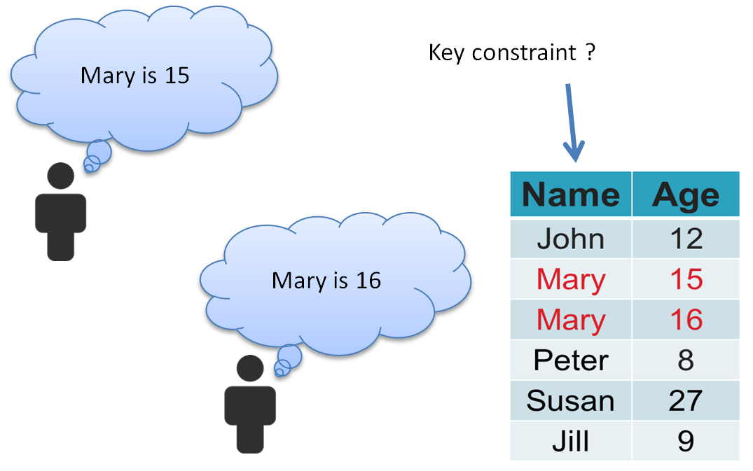
Imposing a key constraint indirectly solves view update problems, such as
an insertion into a restriction.
Example
Consider the following relation R which violates the FD: {X}→{Y}
(see functional dependency []).
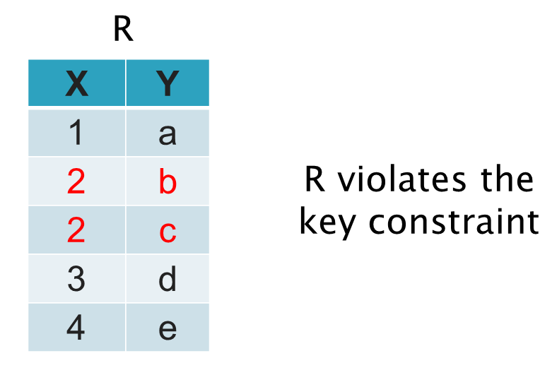
We would like to impose the key constraint expressed by the FD {X}→{Y}, but only indirectly.
Remove duplicates to satisfy the key constraint
Consider that a derived variable K is defined using a relational algebra expression on R
such that K contains the tuples from R without the duplicates.
Therefore K satisfies the key constraint:
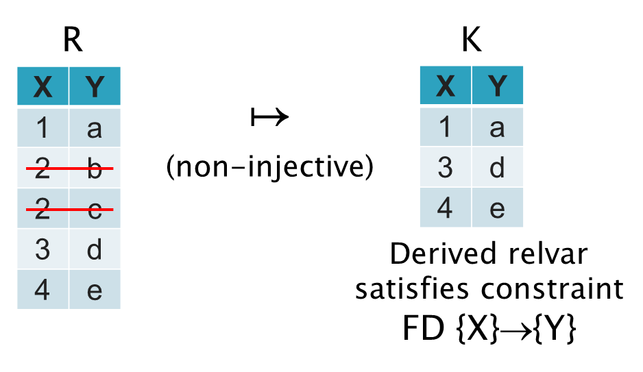
Can derive the offending tuples (highlight "errors" to users)
Consider that a derived variable D is defined using a relational algebra expression on R
such that D contains the duplicates from R:
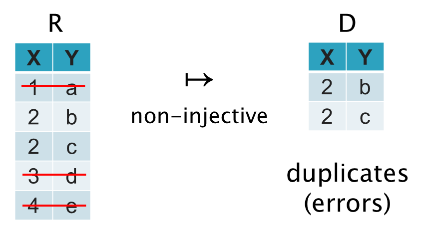
Can materialise a bijective representation
There is a bijection between R and (K,D). Therefore we can consider the pair (K,D) to be an alternative
representation of the information in R.
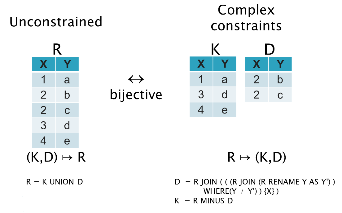
Indeed it is appropriate for the physical implementation to materialise the representation (K,D)
instead of R, because it is cheaper to calculate R from (K,D) rather than the reverse.
Nevertheless R is regarded as the more appropriate representation for expressing updates,
since it is unconstrained, whereas (K,D) have complicated constraints.
The representation R is also more appropriate for allowing Operational Transformation to be used to merge
concurrent updates.
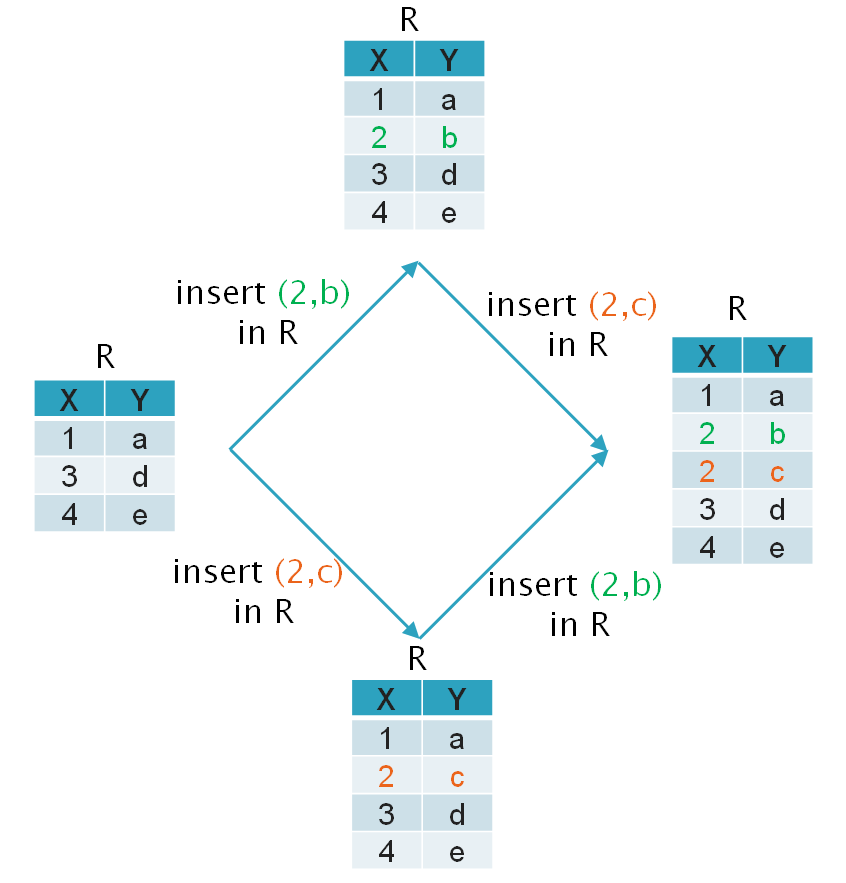
Operational Transformation on R
Since R is unconstrained, it is relatively easy to merge concurrent operations. For example, insert
operations on sets commute, so therefore:
Operational Transform on (K,D)
Much of the literature on Operational Transformation is concerned with finding inclusion transforms
that satisfy properties TP1 and TP2, which are needed to ensure all sites converge at quiescence.
See this primer on Operational Transformation
It is not easy, indeed there have been many examples of erroneous algorithms, one research group
proposed using automated theorem provers to validate the solutions.
See
Proving correctness of transformation functions in collaborative editing systems by
Gérald Oster, Pascal Urso, Pascal Molli and Abdessamad Imine (2005).
Trying to make Operational Transformation work with updates on K,D directly, while satisfying the
transformation properties TP1 and TP2 appears like a hard problem, the solution indeed looks
complicated:
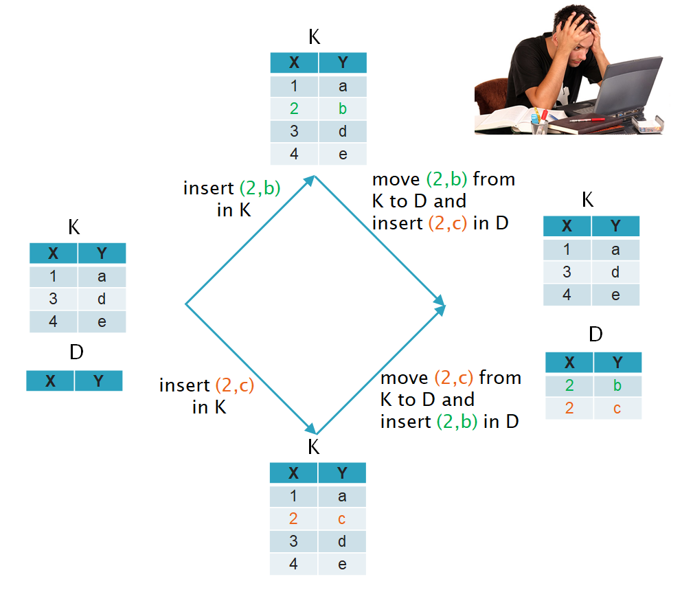
Note for example that inserting a tuple in R might do something relatively complicated on K and D.
E.g. it may cause a tuple to be moved from K to D (a tuple is removed from K and two tuples are inserted in D).
The math leads to interesting update operations on the representation using K,D in
such a way that the FD constraint on K is imposed even as we merge concurrent operations.
Empty key
Declaring a relvar to have an empty key imposes the constraint that its cardinality doesn't
exceed one.
A relvar with an empty key cannot have any other keys defined - because it is never the case
that a candidate key is a strict subset of another candidate key (candidate keys are irreducible).
27 Information equivalence classes
Two schemas are information equivalent if they represent the same information.
Let `W` denote the set of possible world situations, and let `S` be a relational database schema.
Let `d_S(w)` denote the database value for schema S in world situation `w∈W`.
Let `D(S)` = `{ d_S(w) | w∈W }` denote the set of possible database values with schema `S`.
It is assumed `D(S)⊆C(S)` - i.e. the constraint doesn't prevent the recording of possible
world situations.
We say the database constraint of `S` has been specified maximally if `C(S) = D(S)`.
Definition: We say the information in schema `S_1` contains the information in schema `S_2`
if
`∀w,w'∈W: (d_(S_1)(w)=d_(S_1)(w')) → (d_(S_2)(w)=d_(S_2)(w'))`
Definition: We say `S_1` and `S_2` are information equivalent
if each contains the information in the other.
This relation is reflexive, symmetric and transitive, and is therefore an equivalence relation.
Therefore database schemas are partitioned into information equivalence classes.
The business requirements determine the information to be recorded which in
turn determines all the following:
- the information equivalence class
- the "maximal" constraint on each schema within the information
equivalence class
- what facts can be asserted independently of other facts
Maximal decomposition of information
For a given information equivalence class and constraint, it can be shown there always
exists a schema which achieves the maximal partition of its relvars into groups
which can be updated independently.
See maximal decomposition of information.
Interestingly this maximal decomposition corresponds to the unique prime
factorisation of the number of possible database values `N = |C(S)|`.
Do we expect that in real database systems `N` tends to be a large prime number?
It would be surprising if the number of states defined by real-life database
schemas (with maximal constraints) tend to be prime numbers.
It's difficult to think of a reason to expect it given that the
Prime Number Theorem []
says large primes are much less common than large composites, and given that in
mathematics/computing it is generally a hard problem to find large prime
numbers, despite number theorists thinking about the problem for a long time.
It seems likely that in practise for real databases with
finite types the number of prime factors is very large despite the constraints.
Perhaps this isn't apparent because of the tendency to not consider designs
having Database-Valued-Attributes (DVAs) (which goes against Codd's idea of simple
attribute types).
Normalisation
Normalisation is concerned with identifying a schema within an equivalence
class which is more convenient to use in some sense. It doesn't affect what
facts can be asserted or retracted independently of other facts.
It would be interesting to know how nornalisation relates to maximal decomposition
as defined above.
28 Unique prime Cartesian factorisation of a relation
Let 1 denote the relation DEE
which represents the identity for Cartesian product. A prime relation
is a non-empty relation not equal to 1 which can only be Cartesian-factorised into
1 and itself.
A prime relation is analogous to a prime number, including the notion of a unique prime factorisation.
In number theory, the unique prime factorisation of the integers greater than
0 is such an important theorem that it is referred to as the
Fundamental theorem of arithmetic [].
Theorem: every non-empty relation R has a unique prime Cartesian factorisation:
\(R = R_1 ⨯ R_2 ⨯ ... ⨯ R_n\)
\(R_1,...,R_n\) are the prime factors of \(R\).
If \(R\) is infinite then at least one of the prime factors is infinite.
In the following example \(R_1\) and \(R_2\) are the prime factors of \(R\).
| \(R\) |
\(=\) |
\(R_1\) |
\(⨯\) |
\(R_2\) |
| var1 | var2 | var3 |
|---|
| a | 1 | x | | a | 2 | x | | b | 1 | x | | a | 1 | y | | a | 2 | y | | b | 2 | y |
|
|
|
|
|
No equivalent for natural join
It's clear that this doesn't apply to joins (even though join generalises
Cartesian product and is also commutative and associative and has identity
DEE). For example, the fact that \(r⋈r = r\) is a showstopper. By contrast,
Cartesian product forces the factors to be "smaller" because the factors involve
a partitioning of the set of attributes, and it is noteworthy that something
along these lines is used in Euclid's proof that there exists a prime
factorisation of any integer. However the proof assumes integers are
well-ordered which doesn't apply to relations, so the proof doesn't apply as
written.
Proof
The proof is reasonably
complex. It makes use of many properties of the relational algebra, and the
fact that the naturals are well-ordered. There is a proof that a prime
factorisation exists and a proof that it is unique if it exists.
29 Proof of the unique prime Cartesian factorisation of a relation
The proof can be split into two parts:
- a proof that a prime factorisation exists; and
- a proof that it is unique if it exists.
This treatment assumes an
untyped formalism of relational theory.
Relations are modelled as a set of tuples (without any separate notion of a header, nor
with any notion of types of attributes) and therefore the empty relation is the
empty set ∅, and DEE={∅} is the relation containing a single empty tuple.
Attributes of a relation
In this proof we are typically only concerned with non-empty relations, and
therefore the set of attributes of the relation is uniquely defined.
Def: For any relation r≠∅, let *r denote the set of attributes of relation r.
Note: *∅ represents the attributes of the empty relation and is undefined.
Note: To avoid excessive bracketing we assume the unary prefix operator * has
higher precedence than infix operators.
Projection
Def: The projection of relation r on any set of attributes α is denoted by r[α].
To avoid excessive bracketing we assume the unary postfix operator [] has higher
precedence than infix operators.
Note: If r≠∅ then *(r[α]) = *r ∩ α.
Note: Let r be any relation and α,β be any sets of attributes, then r[β][α] = r[α∩β].
Cartesian product
Def: Let r and s be relations. We write r⊥s if it is not the case that r and
s are non-empty relations with common attributes. i.e.
r⊥s = ¬( r≠∅ ∧ s≠∅ ∧ (*r∩*s)≠∅ )
Note: If r⊥s then the join r⋈s represents a Cartesian product, which we
denote more specifically by r⨯s.
Note:
if r⊥s then r⨯s = s⨯r
if r⊥s and s⊥t then (r⨯s)⨯t = r⨯(s⨯t)
Note: Let r and s be non-empty relations with r⊥s. Then *(r⨯s) = *r ∪ *s X1
Note: Let r and s be relations with r⊥s. Then (r⨯s = ∅) ⇔ (r=∅ ∨ s=∅) X2
Note: Let r and s be non-empty relations with r⊥s. Then (r⨯s)[*r] = r X3
Note: Let r and s be non-empty relations with r⊥s and α be any set of attributes. Then:
*r ∩ α = ∅ ⇒ (r⨯s)[α] = s[α]
(*r ∩ α ≠ ∅) ∧ (*s ∩ α ≠ ∅) ⇒ (r⨯s)[α] = r[α] ⨯ s[α] X4
Claim: If r,s,t are relations with r≠∅, r⊥s and r⊥t, then (r⨯s = r⨯t) ⇒ s=t X5
Proof:
Suppose not. i.e. r≠∅, r⨯s = r⨯t and s≠t
if s=∅ then
r⨯t = ∅ (because r⨯t = r⨯s = r⨯∅ = ∅)
t=∅ (by X2 and r≠∅)
contradicts s≠t
else
s≠∅
if t=∅ then
r⨯s = ∅ (because r⨯s = r⨯t = r⨯∅ = ∅)
s=∅ (by X2 and r≠∅)
contradicts s≠∅
else
t≠∅
*r ∪ *s = *(r⨯s) (by X1)
= *(r⨯t)
= *r ∪ *t (by X1)
(*r ∪ *s) \ *r = (*r ∪ *t) \ *r (subtract *r from both sides)
(*r\*r) ∪ (*s\*r) = (*r\*r) ∪ (*t\*r) (set difference is right
distributive over union)
*s\*r = *t\*r (*r\*r = ∅)
*s = *t (*r ∩ *s = ∅ and *r ∩ *t = ∅)
s = (r⨯s)[*s] (because r≠∅ and s≠∅ and by X3)
= (r⨯t)[*t] (substitute r⨯s = r⨯t and *s=*t)
= t (because r≠∅ and t≠∅ and by X3)
contradicts s≠t
Identity of Cartesian product
Def: Let 1 denote the relation {∅} (i.e. DEE). I1
Note: ∀r, r⨯1 = 1⨯r = r. I2
Note: if r≠∅ then (*r=∅ ⇔ r=1) I3
Cartesian product on a set of relations
Def: Let R be a finite set of relations with no attributes in common between
any pair of non-empty relations within R. i.e. ∀r,s∈R, r⊥s. ∏(R) denotes
the Cartesian product of all relations in R, with special cases
∏(∅) = 1 and ∀r, ∏({r}) = r. M1
Note: ∏(R) is well defined because the Cartesian product is commutative and
associative.
Note: ∀R,S, ∏(R∪S) = ∏(R) ⨯ ∏(S) M2
Note: ∏(R)=∅ ⇔ ∅∈R M3
Degree of a relation
Def: For any relation r≠∅, let deg(r) = |*r|. deg(∅) is undefined. DEG1
Note: Let r and s be non-empty relations with r⊥s. Then deg(r⨯s) = deg(r) + deg(s) DEG2
Prime relations
Def: Relation r is prime if both the following hold: P1
- r ≠ 1; and
- r = s⨯t ⇒ {s,t} = {1,r}
Note: ∅ is not prime P2
Prime factorisation of a relation
Def: Let r be a relation and R be a set of relations. P3
R is a prime factorisation of r if both:
- r=∏(R) ; and
- ∀s∈R, s is prime
Note: Relation ∅ has no prime factorisation. P4
Note: 1 has a prime factorisation ∅ since ∏(∅)=1 P5
Note: Every prime relation r has a prime factorisation {r} since ∏({r})=r. P6
Existence of prime factorisation of every non-empty relation
Note: Less than (<) on the natural numbers N = {0,1,2,... } is a well-order
relation. < is a strict total order with the property that every non-empty
subset of N has a least element in this ordering.
Claim: ∀ relation r≠∅, ∃ prime factorisation R of r. E1
Proof:
Suppose not. Then there exist one or more non-empty relations with no prime
factorisation.
The natural numbers are well ordered. Therefore there must exist a smallest
degree for relations with no prime factorisation.
Let it be n.
Let r be a relation with deg(r)=n and r has no prime factorisation, and every
relation of degree less than n has a prime factorisation.
Suppose n=0.
Then deg(r)=0 so r=1.
But 1 has a prime factorisation ∅ since ∏(∅)=1.
This contradicts our supposition that r has no prime factorisation, so n>0.
Suppose r is prime.
Then r has a prime factorisation {r} since ∏({r})=r.
This contradicts our supposition that r has no prime factorisation, so r
cannot be prime.
So we can assume both r is not prime and r≠1.
Therefore ∃s,t such that r=s⨯t and {s,t}≠{1,r}.
From r=s⨯t we know n = deg(r) = deg(s)+deg(t).
Suppose s=1. Then r = s⨯t = 1⨯t = t. This contradicts {s,t}≠{1,r}, therefore s≠1.
Suppose t=1. Then r = s⨯t = s⨯1 = s. This contradicts {s,t}≠{1,r}, therefore t≠1.
Since s≠1, deg(s)>0. From n = deg(s)+deg(t) we deduce deg(t)<n.
Since t≠1, deg(t)>0. From n = deg(s)+deg(t) we deduce deg(s)<n.
By supposition every relation of degree less than n has a prime factorisation.
Therefore ∃prime factorisation S of s, and ∃prime factorisation T of t.
Therefore s=∏(S) and t=∏(T).
Now ∏(S∪T) = ∏(S)⨯∏(T) = s⨯t = r.
Also ∀u∈S∪T, u is prime (since all members of both S and T are prime).
Therefore S∪T is a prime factorisation of r.
This contradicts our supposition that r has no prime factorisation.
Divides
Def: Let r and s be relations. We write r|s meaning r divides s if ∃t, r⨯t = s D1
Note: ∀r r|∅. (and in particular ∅|∅) D2
Note: Let r≠∅ and s≠∅. Then r|s ⇒ r=s[*r] D3
Note: ∀r r|r. D4
Note: ∀r 1|r. D5
Note: ∅|r ⇒ r=∅ D6
Uniqueness of prime factorisation of a relation
Lemma: Let p and r be non-empty relations. Then:
(*p ⊂ *r) ∧ (∃ t≠∅, (p|t) ∧ (r|t)) ⇒ p|r U1
(note that the strict subset operator is used in the condition *p ⊂ *r)
Proof:
Suppose p≠∅, r≠∅, *p⊂*r, t≠∅, p|t, r|t. We want to prove p|r.
if *p=∅ then
p=1 (by I3)
1|r (by D5)
p|r (substitute p=1)
else
*p≠∅
p≠1 (otherwise *p=∅)
r≠1 (otherwise *r=∅ contradicting *p⊂*r)
∃s r⨯s = t (from r|t and D1)
∃q p⨯q = t (from p|t and D1)
s≠∅ (otherwise t = r⨯s = r⨯∅ = ∅, contradicting t≠∅)
q≠∅ (otherwise t = p⨯q = p⨯∅ = ∅, contradicting t≠∅)
*s⊂*q (because
*p⊂*r
(*t\*r) ⊂ (*t\*p) (take complement w.r.t. *t on each side)
*s = *t\*r (because *t = *r∪*s and *r∩*s = ∅)
*q = *t\*p (because *t = *p∪*q and *p∩*q = ∅)
*s⊂*q (substitutions in (*t\*r) ⊂ (*t\*p))
)
if *s ∩ *q = ∅ then
*s=∅ (*s⊂*q and *s∩*q = ∅)
s=1 (s≠∅, and *s=∅ so can apply I3)
r = p⨯q (r = r⨯1 = r⨯s = p⨯q)
p|r (by D1)
else
*s∩*q ≠ ∅
*r∩*q ≠ ∅ (because
*q = *t\*p (because *t = *p∪*q and *p∩*q = ∅)
= (*r∪*s) \ *p
= (*r\*p)∪(*s\*p) (set difference is right
distributive over union)
*r\*p ⊆ *q (property of set union: A⊆(A∪B))
*r\*p ⊆ *r (property of set difference: (A\B)⊆A)
*r\*p ≠ ∅ (*p ⊂ *r)
*r ∩ *q ≠ ∅ (From above 3 facts about *r\*p)
)
q = (p⨯q)[*q] (by X3 since p≠∅ and q≠∅)
= (r⨯s)[*q] (substitute p⨯q = t = r⨯s)
= r[*q]⨯s[*q] (by X4 since *r∩*q≠∅ and *s∩*q≠∅)
= r[*q]⨯s (*s⊂*q so s[*q]=s)
r⨯s = p⨯q
= p⨯(r[*q]⨯s) (substitution for q)
= (p⨯r[*q])⨯s (by associativity of ⨯)
p ⨯ r[*q] = r (s≠∅ so apply X5)
p|r (by D1)
Lemma: ∀prime relation p, ∀r,s with r⊥s, p|(r⨯s) ⇒ (p|r)∨(p|s) U2
Proof:
Suppose p is prime, r⊥s, and p|(r⨯s). We shall show (p|r)∨(p|s)
if r=∅ then
p|∅ (by D2)
p|r (substitute r=∅)
else if s=∅ then
p|∅ (by D2)
p|s (substitute s=∅)
else if r=1 then
r⨯s = 1⨯s = s
p|s (substitute r⨯s=s in p|(r⨯s))
else if s=1 then
r⨯s = r⨯1 = r
p|r (substitute r⨯s=r in p|(r⨯s))
else
r≠∅, s≠∅, r≠1, s≠1
r⨯s ≠ ∅ (by X2)
∃q, r⨯s = p⨯q (p|(r⨯s) and D1)
p≠∅, q≠∅ (otherwise r⨯s = p⨯q = ∅, contradicting r⨯s ≠ ∅)
if *p ⊂ *r then
∃ t≠∅, (p|t) ∧ (r|t) (let t = r⨯s = p⨯q)
p|r (by U1)
else if *p⊂*s then
∃ t≠∅, (p|t) ∧ (s|t) (let t = r⨯s = p⨯q)
p|s (by U1)
else if *p=*r then
r = (r⨯s)[*r] (by X3)
= (p⨯q)[*p] (substitute *p = *r and p⨯q = r⨯s)
= p (by X3)
r|r (by D4)
p|r (substitute r=p)
else if *p = *s then
s = (r⨯s)[*s] (by X3)
= (p⨯q)[*p] (substitute *p=*s and p⨯q = r⨯s)
= p (by X3)
s|s (by D4)
p|s (substitute s=p)
else
*p⊄*r, *p≠*r i.e. ¬(*p⊆*r)
*p⊄*s, *p≠*s i.e. ¬(*p⊆*s)
*r∩*p ≠ ∅ (because ¬(*p⊆*s))
*s∩*p ≠ ∅ (because ¬(*p⊆*r))
p = (p⨯q)[*p] (by X3)
= (r⨯s)[*p] (substitute r⨯s = p⨯q)
= r[*p] ⨯ s[*p] (*r∩*p ≠ ∅ and *s∩*p ≠ ∅ so apply X4)
contradicts p is prime (p has been factorised into r[*p]⨯s[*p])
Claim: ∀relation r≠∅, prime factorisation of r is unique U3
Proof:
Suppose not.
Then there are non-empty relations with distinct prime factorisations.
Let n be the smallest degree of any such relation.
Let t≠∅ be a relation of degree n with prime factorisations P and Q with P≠Q.
t = ∏(P) = ∏(Q)
P≠∅ (otherwise t=∏(P)=1 which has unique factorisation ∅)
∃p∈P (because P≠∅)
Q≠∅ (otherwise t=∏(Q)=1 which has unique factorisation ∅)
∃q∈Q (because Q≠∅)
Let q' = ∏(Q\{q})
t = ∏(Q) = q⨯∏(Q\{q}) = q⨯q'
n = deg(t) = deg(q)+deg(q') (by DEG2)
deg(q')<n (because deg(q) > 0 since q∈Q is prime)
q' has unique prime factorisation (deg(q') < n and definition of n)
p | (q⨯q') (because p∈P so p|∏(P) and ∏(P) = q⨯q')
(p|q)∨(p|q') (p is prime so lemma U2 is applicable)
Claim: p∈Q
Proof:
if p|q then
p=q
p∈Q
else
p|q' (because (p|q)∨(p|q'))
∃u p⨯u = q' (by D1)
u≠∅ (otherwise q'=∅ so t=∅)
∃U U is prime factorisation of u (by E1 and u≠∅)
q' = p⨯u = p⨯∏(U) = ∏(U∪{p})
U∪{p} = Q\{q} (q' has unique prime factorisation)
p∈Q
Let t' = ∏(P\{p}) = ∏(Q\{p}).
t = p⨯t' (by M2)
n = deg(t) = deg(p)+deg(t') (by DEG2)
deg(t')<n (p is prime so deg(p)>0)
t' has unique factorisation (deg(t')<n and definition of n)
P\{p} = Q\{p} (because t' has unique factorisation)
P=Q (otherwise P\{p} ≠ Q\{p})
Contradiction to P≠Q
30 Independently updatable variables
Let information be recorded in a set of variables, and there are declared integrity constraints on
these variables. We say a variable is independently updatable if the set of possible
values of that variable (as determined by the constraint) is independent of the values
of the other variables.
For the purpose of investigating independently updatable variables we are not interested in
alternative ways of changing a variable (e.g. UPDATE versus INSERT versus DELETE on a relvar).
Instead we are going down to a finer-grained level so we can talk about variables which can
be assigned any value of their type.
In other words we’re tending to (where we can) uphold a principle:
To be an updatable variable of type T is to support assignment of any value of type T.
or
To be an updatable variable is to be an independently updatable variable.
If a variable is not independently updatable we’re tending to ignore it being available as the
denoted target for update operations.
Example
For example suppose relation R represents the extension of the integrity constraint on variables
var1,var2, var3.
This is the set of possible (i.e. valid) states of variables var1, var2, var3.
It can be proven that every nonempty relation has a
unique prime Cartesian factorisation.
In this case R = R1⨯R2. R1 and R2 are the prime factors of R.
| R |
= |
R1 |
⨯ |
R2 |
| var1 | var2 | var3 |
|---|
| a | 1 | x | | a | 2 | x | | b | 1 | x | | a | 1 | y | | a | 2 | y | | b | 2 | y |
|
|
|
|
|
The unique prime Cartesian factorisation implies there is a unique maximal
partition of the variables into groups which can be updated independently.
This partition is uniquely determined by the constraints. Complicated constraints
mean fewer groups and less opportunity for updating variables independently.
In this case {var1,var2,var3} is partitioned into two sets: {var1,var2} and {var3}.
The prime Cartesian factorisation of the extension of a constraint
There is a
unique prime Cartesian factorisation (PCF)
of any non-empty relation.
In the following we are interested in the PCF of the extension of a possrep constraint.
There is a unique PCF of the extension of a given possrep constraint, the effect
being to partition the possrep components so that the components within one factor
can be updated independently of the other factors - i.e. there are no constraint
dependencies between factors.
Note that a unique PCF exists for both finite and infinite non-empty relations, so for
example it is applicable to constraints in computational geometry examples involving
infinite sets in Euclidean space. Of course that involves intensional definitions of
sets.
For example it is easy to see that we can factorise
`{ (x,y,z) ∈ ℝ^3 | x^2+y^2=1 ∧ z>0 }`
as
`{ (x,y) ∈ ℝ^2 | x^2+y^2=1 } ⨯ { (z) ∈ ℝ | z>0 }`
The way in which constraints can be expressed is open ended. In the context of
mathematical computing, data structures and algorithms in general (not just the
trivial finite relations), it would be interesting know whether in general if one
splits a representation into two parts with no mutual constraints, can it be
assumed this particular division is compatible with the maximal way of splitting
the representation into many parts with no mutual constraints? Intuitively it
seems plausible but can it be proven? That is the purpose of the unique PCF
theorem.
The unique PCF theorem (which is an existence & uniqueness proof) is what allows
one to give a formal definition of the unique maximal partition of variables
into groups which can be updated independently. It therefore provides an objective
metric for selecting between alternative representations.
It shows that in general constraints on a tuple no matter how complex can be
uniquely written in a normalised form as a conjunction where the extension of
each conjunct is a prime Cartesian factor of the extension of the entire constraint.
Here we are only talking about a normal form modulo how the conjuncts are
expressed. This normal form sounds vaguely like Conjunctive Normal Form (CNF)
but it's not the same thing.
It is conjectured that the normal form is very important to high performance dbms
implementation technique (it relates to asynchronous updates, locking and
concurrency, replication and synchronisation, branching and merging, constraint
checking, ...)
We shall abuse terminology and talk about the information recorded in a prime
factor, which really means the information recorded by the attributes in that
factor. There are some general statements that can be made in this regard.
For example, prime factors relate to units of cohesion. i.e. there is some
sense in which information within a prime factor is mutually interdependent
and indivisible, whereas between different prime factors the information is
more independent, and provides a basis for supporting independent and
concurrent data entry by different users. That means it is a relevant to data
representation independence and updateable views. If a representation provides
many prime factors then it is expected there are more opportunities for
choosing where and what information is visible and/or updatable. This translates
into better support for data representation independence.
Prime factors are also relevant to locking and concurrency, and the granularity
of atomic updates. For example, if we define atomic updates to be the most
primitive updates that are compatible with integrity preservation, then clearly
that idea is somehow connected to prime factors. It follows that prime
factors might be relevant to scalability of databases. If very large databases
don't have prime factors then atomic updates might be complex, take longer to
execute, are more difficult to validate and concurrency might be limited.
This is particularly relevant to distributed databases - e.g. it might be
preferable for prime factors to not be distributed over a network to avoid the
need for distributed atomic commit protocols.
If prime factors are indeed an important consideration, it's nice to know that
they are defined uniquely and independently of the way integrity constraints
happen to be expressed in the schema (e.g. uniqueness constraint, functional
dependency, foreign key constraint, or some boolean valued expression making
use of the relational algebra). Prime factors provide some basis for
comparing alternative data representations.
The prime factors on the database tuple of a relational database represent a
fairly coarse partition of a large schema into independent parts, and therefore
only appears to have limited utility.
However, later in this paper we discuss the idea that a database can typically
be factored into a much larger set of conditionally existent prime factors.
If prime factors are small enough, then it is possible that a system with
MVCC + one write mutex per factor, has advantages over conventional strict 2PL
lock managers with dead-lock detection etc. What's the point in burdening
the lock manager with support for concurrent updates within a factor within
which values have a bearing on each other - as far as constraint checking is
concerned?
todo
The effect is to partition the attributes of the relation into non-empty subsets. A projection gives the potential factors.
Note that the motivation is not to factorise the relations recorded in a database! Instead the intended
application is the prime factorisation of the relation which is the set of tuples on which a constraint is imposed on a
representation of a value of a given type using a tuple.
The idea is to define mathematically what it means exactly for relvars to be "connected" given the database constraints, in the sense
of partitioning them into groups that can be updated independently.
The constraints on the dbvar determine a set of dbvalues which satisfy the constraints. This is a set of tuples. In fact it is a
non-empty relation which has a unique prime Cartesian factorisation. This gives the partition of the relvars into mutually
"connected" groups
31 Maximal decomposition of information
Let `S` be a relational database schema.
`C(S)` (the extension of the database constraint) can be regarded as a non-empty relation so we can consider its
unique prime Cartesian factorisation.
Claim:
For any schema `S` there exists a schema `S'`
which is information equivalent to `S`
where the cardinality of every finite prime Cartesian factor of `C(S')` is a prime number.
This implies the bag of integers which are the cardinalities of the prime
Cartesian factors of `C(S')` equals the bag of prime number factors of `|C(S)|`.
Note that the bag of prime number factors of any positive integer is uniquely determined, by
the Fundamental theorem of arithmetic [].
`S'` represents a schema having maximal decomposition - i.e. into the most parts which can be updated
independently.
Proof
The following is an outline of a constructive existential proof which involves
relational expressions for each relvar in `S'` that are defined in terms of the
relvars of `S`:
Let `F_1, ..., F_n` be the prime number factors of `N = |C(S)|` (the order doesn't matter)
Let the `N` database values in `C(S)` be organised into an `n` dimensional array of size
`prod_(j=1)^n F_j = N` (again, the order doesn't matter).
For `j` in `1..n` and `i` in `1..Fj`,
let `B_(ij)` denote the subset of `C(S)` corresponding to the set of database values in
the ith slice of the jth component of the n-dimensional array
(a slice has `n-1` dimensions).
For `j` in `1..n` and `i` in `1..F_j`, let `T_(ij) = uuu { matches(d) | d ∈ B_(ij) }`
where `matches(d)` evaluates to DEE if the dbvar for schema `S` has value
`d`, otherwise DUM. See how it can be defined here.
Note that `T_(ij)` evaluates to DEE if the value of the dbvar for `S` is in slice `B_(ij)`, otherwise DUM.
Let `x` be some attribute name.
For `j` in `1..n`,
let schema `S'` have relvar `R_j'` which is defined in terms of the relvars of `S` using
the expression
`R_j' = uuu { T_(ij) ⋈` REL { TUP { (`x` `i`) } }` | i in 1..F_j }`
(this expression evaluates to REL { TUP { (`x` `i`) } } where the dbvar of
`S` is in slice `B_(ij)`)
Note that for every database value each relvar `R_j'` of `S'` has exactly one tuple with one
attribute. This follows because any database value (i.e. element of `C(S)`) lies in
exactly one slice of the jth coordinate. The UNION over the JOINs picks out
exactly one of the TUP { (`x` `i`) }. There are `F_j` slices for the jth component
and hence `F_j` possible values of `R_j'`.
It is easy to see that a combination of the values of the `R_j'` corresponds to
one of the elements of the n-dimensional array and hence to one of the database values
in `C(S)`.
Example 1
Let there be three lights coloured red, green and blue which can be on or off.
There are `2^3 = 8` world situations which need to be recorded.
Let schema `S_1` have a single relvar with the predicate:
The light with colour [COLOUR] is on.
Let schema `S_2` have three relvars with the following predicates:
- The red light is on.
- The green light is on.
- The blue light is on.
`S_1` and `S_2` are information equivalent. `S_2` is an example of a schema with maximal decomposition.
Example 2
Let there be three lights coloured red, green and blue which can be on or off,
except they cannot be all off or all on.
There are `6` world situations which need to be recorded.
The prime factorisation of `6` is `2×3`.
A maximally decomposed schema can be achieved with the following two predicates:
- A single light is on.
- The light with colour [COLOUR] is the only light in its state.
Example 3
See maximal decompositon of two monadic relations with an IND constraint.
32 Two monadic relations with an IND constraint
This example illustrates the
maximal decompositon
of two monadic relations with an IND constraint.
Let \(T\) be a finite type where there are \(n\) values of type \(T\).
Let schema \(S\) have two relvars \(R_1\), \(R_2\) each
having the same single attribute of type \(T\) and there's an Inclusion Dependency (IND)
constraint defined: \(R_2⊆R_1\).
The number of ways we can have \(i\) tuples in \(R_1\) is \(\binom{n}{i}\).
For \(i\) tuples in \(R_1\) the number of subsets of those tuples which can appear
in \(R_2\) is \(2^i\).
Therefore the number of possible database values is \(\displaystyle|C(S)| = \sum_{i=0}^{n} \binom{n}{i} 2^i\).
Example with n=2
With \(n=2\), we get
\(|C(S)| = \binom{2}{0}2^0 + \binom{2}{1}2^1 + \binom{2}{2}2^2
= 1 + 4 + 4
= 9\).
Let the two values of \(T\) be \(a\) and \(b\).
We can denote values of the relations \(R_1\) and \(R_2\) by subsets of \(\{a,b\}\)
according to which tuples are present.
The following table shows the \(9\) possible database values which satisfy the IND constraint:
| R1 | R2 |
|---|
| {} | {} |
| {a} | {} |
| {a} | {a} |
| {b} | {} |
| {b} | {b} |
| {a,b} | {} |
| {a,b} | {a} |
| {a,b} | {b} |
| {a,b} | {a,b} |
Cartesian factorisation of the information in the database
It just so happens that the expression for the number of possible database values can be simplified:
\(\displaystyle|C(S)| = \sum_{i=0}^{n} \binom{n}{i} 2^i = 3^n\).
(e.g. for \(n=2\) we have \(3^2 = 9\) database values.
For \(n=3\) we get \(3^3=27\), For \(n=4\) we get \(3^4 = 81\) and so on).
This can be proven with the binomial theorem. It gives us the prime number factorisation of \(|C(S)|\).
There is a corresponding schema \(S'\) which is
information equivalent to \(S\) involving \(n\) relvars
for the \(n\) values of type \(T\). These relvars can be updated independently.
Each relvar implicitly refers to one of the values of type \(T\) and has exactly \(3\) possible values:
- the value isn't present in either \(R_1\) or \(R_2\)
- the value is present in \(R_1\) but not \(R_2\)
- the value is present in both \(R_1\) and \(R_2\)
Note that these propositions treat the value as implied, in exactly the manner
discussed with nested databases.
In practise \(n\) can be very large. For example \(n = 2^{64}\) if \(T\) is a 64 bit integer.
Obviously we can't expect a system to physically represent \(2^{64}\) relvars.
In fact a vast number of independently updatable variables is good.
The maximal decomposition tells us what can be independently updatable in some logical
representation, and more specifically for having expressions which denote variables which
are the target of updates. It is not prescribing a physical implementation.
33 Unrolling a predicate
Consider the maximal decompositon of two monadic relations with an IND constraint.
This simple example illustrates an "unrolling" technique of "partially/fully instantiating"
predicates to obtain larger numbers of predicates for a different representation of the same
information (i.e. a representation that is
information equivalent).
The "unrolling" is just a conceptual technique to find parameterised expressions
which denote derived relvars which are suited to be the target of updates.
It should not be taken to mean that actual database schemas will be expressed in
the unrolled form.
See the S&P
example for a more complex/realistic example with INDs.
34 Factorisation of supplier and parts database schema
The supplier-and-parts database schema appears in Chris Date's book
An introduction to Database Systems.
There are three relvars in the schema, used to represent suppliers, parts and shipments.
It is a conventional normalised relational database schema.
Note that if one puts this schema into 6NF there are 8 instead of 3 relvars.
Even in 6NF form none of the relvars are
independently updatable.
We will now consider an alternative
information equivalent schema
using a nested relational database schema, meaning there are
Database Valued Attributes (DVAs).
In other words there are relational database values appearing as attribute values
within a containing relational database.
The "nesting" is a technique that can be used in a real schema definition to
help organise the information in a way that highlights orthogonality.
The advantages in terms of a separation of concerns, orthogonality of information and independent
updates is discussed.
See nested databases.
The key idea is to regard a relational database schema as a
possrep defining a type (a dbtype).
Supplier Database
A SUPPLIER_DATABASE is a type and represents information about a given supplier.
For example the SUPPLIER_DATABASE for supplier S1 has the following three relvars:
| Relvar |
Predicate |
|
|
the supplier has name [SNAME] |
|
|
the supplier has status [STATUS] |
|
|
the supplier is located in city [CITY] |
These three relvars have the constraint that they have exactly one tuple
(which is equivalent to a constraint that the relvars are non-empty and have empty keys).
They can be updated independently.
Note that these predicates have the form "the supplier ...". They refer
to the supplier with the definite article. So these predicates
presuppose the existence of the supplier, and do not make sense if the
supplier doesn't exist. Putting it another way, the supplier is assumed to
exist in every world situation in which the SUPPLIER_DATABASE has meaning.
Note that even though a supplier number (S#) identifies a supplier, it doesn't
appear as an attribute in any of the relvars of the SUPPLIER_DATABASE.
There is a separation of concerns between identifying the supplier and
representing facts about the supplier. There could be a hundred relvars for
the latter and none of them are concerned with how a supplier is identified.
This is handy when the key is composite or there are multiple candidate keys.
Part Database
A PART_DATABASE is a type and represents information about a given part.
For example the PART_DATABASE for part P1 has the following four relvars:
| Relvar |
Predicate |
|
|
the part has name [PNAME] |
|
|
the part has color [COLOR] |
|
|
the part has weight [WEIGHT] |
|
|
the part is stored in city [CITY] |
These four relvars have the constraint that they have exactly one tuple.
They can be updated independently.
Supplier and parts database
SUPPLIER_DATABASE and PART_DATABASE values can appear as values of attributes
within a SUPPLIER_AND_PARTS_DATABASE.
A SUPPLIER_AND_PARTS_DATABASE is a type and has three relvars:
| Relvar name | Predicate | Key |
|---|
| S | there exists a supplier identified by [S#] described by supplier database [SDB] | {S#} |
| P | there exists a part identified by [P#] described by part database [PDB] | {P#} |
| SP | there exists a supplier identified by [S#] that ships quantity [QTY] of a part identified by [P#] | {S# P#} |
(with the appropriate IND constraints, these three relvars only represent one
Cartesian factor of the possrep components)
Note that these predicates are existentially quantified in concrete parts and
suppliers.
In effect this leads to supplier database variables and part database variables
for each concrete supplier and part that exists.
Note that the creation and destruction of the supplier databases and the part
databases happens through INSERT/DELETEs on the these three relvars.
Unrolling of the supplier and parts database
In the S&P database where there are 5 suppliers, 6 parts and 12 shipments. One
can regard that information as being equivalent to a representation involving
23 independently updatable relvars, using predicate unrolling on the
supplier and part numbers:
- there is a supplier S1 described by supplier database <SDB>
- ...
- there is a supplier S5 described by supplier database <SDB>
- there is a part P1 described by part database <PDB>
- ...
- there is a part P6 described by part database <PDB>
- supplier S1 ships quantity <QTY> of part P1
- ...
- supplier S4 ships quantity <QTY> of part P5
In this representation, we can incorporate the factors in the nested databases
to end up with 5x3 + 6x4 + 12 = 51 variables which can be updated independently.
Can we reasonably say these variables are independently updatable given that
their existence is conditional?
In general we can say: If the variable exists then it is independently updatable.
This idea is not expected to be controversial. E.g. in an dynamically
resizable array the elements are independently updateable if they exist.
FDs and keys
FDs reflect business requirements. The original S&P schema is information
equivalent to the nested schema representation. This implies that the FD’s
have been captured!
In the nested schemas there are still FDs and keys. The original S&P database
which is 5NF has been decomposed into three simpler distinct database schema
which are each in 5NF. Within these simpler schema there are relvars which are
independently updateable, even though there are no independently updatable
relvars in the original schema.
Most of the original FDs are no longer applicable in the nested schemas. For
example the FD {S#}->{CITY} in S is inapplicable because attributes S# and
CITY don't even appear in the same database schema (never mind the same relvar).
Note that the FD {S#}->{CITY} essentially means a supplier is located in
exactly one city. It doesn't imply that the city cannot be updated
independently.
There's a mapping from a set of nested schemas to an information equivalent
unnested schema. The FD {S#}->{CITY} is implied by the nested database schema
because
- There is an FD {S#}->{SDB}
- There is an FD {SDB}->{CITY}
- FDs are transitive
(where SDB is the attribute name for a supplier database - a database which
records information about a single supplier)
(2) holds because
- there is a declared constraint in the supplier database, that there is
exactly one CITY tuple. i.e. The FD {}->{CITY} holds within the
supplier database.
- FDs must be adjusted when they are translated between databases.
The FD {}->{CITY} within the supplier database becomes {SBD}->{CITY}
in the "containing" suppliers and parts database.
Relaxing constraint on city of part
Consider relaxing the FD constraint {P#}->{CITY} - so that a given part can be stored
in at least one city. For example part P1 might be stored at both London and
Paris.
In the nested design it is just a matter of relaxing the constraint on the relvar
that records the cities where a given part is stored:
In the conventional supplier-and-parts database schema
there is far more upheaval to the schema - it is necessary to decompose the parts
relvar P into two relvars, one which records the name, colour and weight
of each part:
| P# | PNAME | COLOR | WEIGHT |
|---|
| P1 | Nut | Red | 12.0 |
| P2 | Bolt | Green | 17.0 |
| P3 | Screw | Blue | 17.0 |
| P4 | Screw | Red | 14.0 |
| P5 | Cam | Blue | 12.0 |
| P6 | Cog | Red | 19.0 |
and another to record the cities (where we can relax the uniqueness constraint on P#):
| P# | CITY |
|---|
| P1 | London |
| P1 | Paris |
| P2 | Paris |
| P3 | Oslo |
| P4 | London |
| P5 | Paris |
| P6 | London |
Also Inclusion Dependency (IND) constraints will need to be added to make sure
the same set of part numbers appear in these two relvars.
Advantages of nested databases
- The nested representation provides a foundation for defining what variables
can be independently updated.
This is needed to allow Operational Transformation to
be used with relational data.
In particular it's needed to get the long list of benefits of CEDA
such as replication and synchronisation.
- The factorisation of the information into different schema can reduce complexity
because they can be designed, specified, documented and understood in isolation.
- Having lots of FDs defined implicitly seems an advantage in complicated
examples.
- There tends to be less upheaval in the schema when FDs change or when primary
keys change.
- A nested physical representation will typically outperform an unnested
representation, and given that today's DBMS products are quite limited with
how well they optimise physical representations, this is useful.
- A nested schema appears to be more flexible in cases where the DVAs are keys.
In that case there doesn't appear to be a mapping to an unnested form without
the introduction of artificial identifiers.
35 Using the PCF to select appropriate representations
Claim 1: A possrep can be formalised as a non-empty relation where
- the components of the possrep are exactly the attributes of the relation;
- the relation is the extension of the possrep constraint (regarded as a predicate parameterised on the attributes); and
- each element of the relation (i.e. tuple) is assumed to represent a value of the type of the possrep. This is similar in nature to a formal semantics.
Claim 2: Every possrep has a well defined prime factorisation
(obviously since every possrep is formalised by a particular non-empty relation)
Claim 3: All things being equal, possreps with more prime factors tend to be more desirable.
Example
Consider a type for geometrical points constrained to an annulus
possrep 1: R1 = { (x,y) ∈ ℝ2 | 1 < x2+y2 < 9 }.
Prime factorisation = {R1}
possrep 2: R2 = { (r,t) ∈ ℝ2 | (1<r<3) ∧ (-π≤t<π) }.
Prime factorisation = {R,T}
where R = { (r) | 1<r<3 } and T = { (t) | -π≤t<π }
An interesting idea is to consider in turn a possrep on each component of a
possrep and so on. Without prejudice from type systems, this provides some basis
for properly maximising the number of prime factors. As a simple example, a
representation of a circle with centre and radius, where the centre can in turn
be represented either by (x,y) or (r,t) coordinates.
It may seem odd to have talked about a type of geometrical point constrained to
an annulus. It's less odd if you consider that such a constraint may exist on an
attribute of a "containing" possrep in which the geometrical point appears. For
example we may be interested in circles centred at positions in an annulus, which
would suggest a representation using (r,t) for the centre of the circle might
be best.
Example
Consider the ellipse E(CX,CY,A,B) with locus
{ (x,y) ∈ ℝ2 | ((x-CX)/A)2 + ((y-CY)/B)2 = 1 }
and the predicate
P(cx,cy,a,b) = the ellipse has centre (cx,cy), major radius a and minor radius b
In the context of the ellipse E(CX,CY,A,B) the predicate P(cx,cy,a,b) has an extension with a single tuple
TUP { <cx CX> <cy CY> <a A> <b B> }
The predicate P(cx,cy,a,b) is equivalent to the conjunction
the centre of the ellipse has x-coord cx AND
the centre of the ellipse has y-coord cy AND
the major radius of the ellipse is a AND
the minor radius of the ellipse is b
If you project away cy,a,b then you get a relation with a single tuple
TUP { <cx CX> }
which is the extension of the predicate
there exists cy,a,b such that
the centre of the ellipse has x-coord cx AND
the centre of the ellipse has y-coord cy AND
the major radius of the ellipse is a AND
the minor radius of the ellipse is b
which is equivalent to
the centre of the ellipse has x-coord cx
because for example
there exists cy such that the centre of the ellipse has y-coord cy
is true.
36 Logical independence
An important feature of a DBMS is to support logical independence.
This allows for immunity of user applications to changes made in the database schema.
Often data tends to be produced by one application and consumed by many more.
Read only views handle logical independence extremely well for the applications that only
read data.
Under the RM, defining a read-only view could hardly be easier - just use the
relational algebra to define derived relvars.
A read only view can involve a non-injective function of the base relvars - i.e. it
can easily remove information, and impose constraints.
A good DBMS will optimise the I/O and caching of the read only views, and allow them to be updated
efficiently with incremental computing.
This is much simpler than for example using ORM to map
relations in the database to objects and writing procedural code to query the objects, cache derived
variables and send messages or implement a bunch of methods of some interface.
In other words logical independence involving stable views is far superior to OO solutions involving
stable message types, or stable interfaces.
View update problem
Logical independence works well for readers but not so well for writers.
This is called the view update problem.
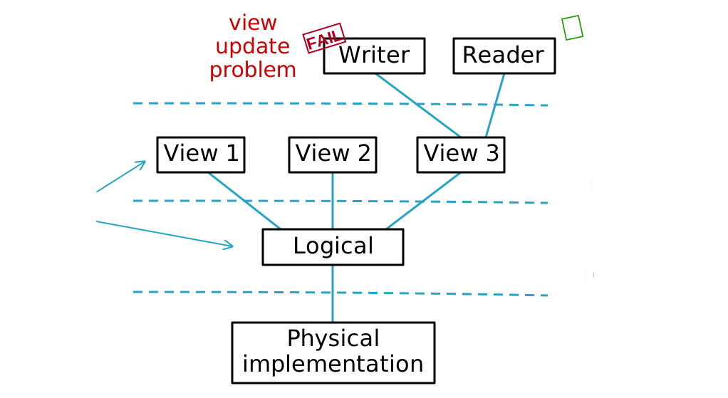
Consider the example of an insert into a restriction.
Part V: Views and updates
This part examines the view-update problem for restrictions, projections and
joins, and develops related principles for interchangeable representations and
relational operations.
37 View update problem
The view update problem refers to the difficulty/impossibility of providing alternative
updatable views on a database.
It's sometimes assumes views are associated with individual relvars.
It's more useful (and more general) to define a view as meaning a derived dbvar.
Therefore a view means a set of named relvars.
(just like the set of base relvars which are defined in the database schema).
It is assumed logical independence implies a view looks and behaves no differently
than if the relvars in the view were declared as base relvars in a schema.
One of the purposes of normalisation is to avoid data redundancy and simpify updating
the database. For that reason it is expected that an updatable view is normalised.
38 Restriction views
To the extent that the base relvars are less constrained, they are more flexible in the
information they can record.
However users probably don't work directly with them.
Instead they work with views which enforce the constraints.
It's asynchronous updates on views which result in temporary offensive tuples in the base
relvars.
I'll illustrate this with an example:
Let B be a base relvar with attributes {X,Y} and no key constraint, even though users
expect the FD {X} --> {Y} according to the predicate.
Let the following views be defined which enforce the key constraint:
    V1 = RemoveDuplicates(B WHERE c, {X})
    V2 = RemoveDuplicates(B WHERE NOT(c), {X})
    V3 = RemoveDuplicates(B, {X})
Let there be a requirement for users to be able to update V1, V2 independently (and asynchronously).
So an assignment to V1 must not change the value of V2, nor can it fail depending on the value of V2.
Proposed solution: an assignment
V1 := NewV1
(where it is assumed all tuples in NewV1 satisfy condition c) updates B according to
B := (B WHERE NOT(c)) UNION NewV1
Note: this assignment can lead to duplicates appearing in B.
This approach supports other conditions for WHERE, giving a great variety of restriction views
which are not always independent (i.e. they can overlap), and yet every view supports well
defined, infallible assignment.
A temporary non-empty (B MINUS V3) is interpreted as a artifact of performing updates on
different views independently and asynchronously.
If we assume every view is eventually assigned correctly according to the extension of its
predicate for a stable world situation, then we expect duplicates in B eventually disappear.
If we assume the views are updated correctly then the database must record the world
situation correctly.
Furthermore V3 provides a relvar which necessarily satisfies the expected constraint,
so V3 can be regarded as the SSOT (Single Source Of Truth) - if an SSOT is needed
at all times - even during periods of change.
The SSOT is accurate to the extent that the users updating the database are accurate.
During periods of change the SSOT is wrong for only as long as the users take to issue
the required updates.
It doesn't make sense that whenever a user performs any update (no matter how small
they would like it to be) they are supposed to ensure that all other outstanding updates
to all relvars are applied as well, in one big synchronous multiple assignment that
might represent thousands of smaller changes.
If a user assigns V2 and is ignorant of V1, then they are authoritative for V2 but
not for V1 or V3.
That seems far more practical than the idea than any user has to correctly and synchronously
update the entire database.
There is no problem with the fact that V1 and V3 are "stale" just after the assignment to V2.
For very big databases a requirement of global synchronous updates depends on the fallacy
that users have access to synchronous snapshots of world situations.
The reality is normally that the information going into a database comes from asynchronous
sources.
The pretense of a database recording a synchronous snapshot of a possible world situation
is ok as long as it is realised that in practice it's just an artifact of what updates have
been applied to the database so far.
If it's an artifact then why not promote efficient, convenient asynchronous updates, and
use a calculation to generate the artifact of a self consistent world situation that appears
to have been recorded in a snapshot - however impossible that might really be?
39 View update problem - insert into a restriction
In the following we discuss an example that appears in chapter 1 of Chris Date's book
View Updating and Relational Theory -
Solving the View Update Problem.
Let S be a base relvar recording suppliers under contract. Each supplier has one supplier number
(SNO), unique to that supplier, one name (SNAME), one status value (STATUS) and one location (CITY).
| SNO | SNAME | STATUS | CITY |
|---|
| S1 | Smith | 20 | London |
| S2 | Jones | 10 | Paris |
| S3 | Blake | 30 | Paris |
| S4 | Clark | 20 | London |
| S5 | Adams | 30 | Athens |
Let LS be a view for the London suppliers defined as a restriction on S where the CITY value is London:
| SNO | SNAME | STATUS | CITY |
|---|
| S1 | Smith | 20 | London |
| S4 | Clark | 20 | London |
Let NLS be a view for the non-London suppliers defined as a restriction on S where the CITY value isn't London:
| SNO | SNAME | STATUS | CITY |
|---|
| S2 | Jones | 10 | Paris |
| S3 | Blake | 30 | Paris |
| S5 | Adams | 30 | Athens |
{SNO} is a key for each of the tables.
{SNO} in each of tables LS and NLS is a foreign key, referencing the key {SNO} in table S.
S and the pair (LS,NLS) are information equivalent meaning there is a
bijective mapping between them.
    S ⟼ (LS,NLS)
        LS = (S WHERE CITY = 'London')
        NLS = (S WHERE CITY ≠ 'London')

    (LS,NLS) ⟼ S
        S = LS UNION NLS
Therefore for any update on S there is an equivalent and uniquely determined update on (LS,NLS) and
vice versa.
This is consistent with the following compensating actions
defined by Chris Date:
    ON DELETE d FROM LS : DELETE d FROM S ;

    ON DELETE d FROM NLS : DELETE d FROM S ;

    ON DELETE d FROM S : DELETE ( d WHERE CITY = ‘London’ ) FROM LS ,
    DELETE ( d WHERE CITY <> ‘London’ ) FROM NLS ;

    ON INSERT i INTO LS : INSERT i INTO S ;

    ON INSERT i INTO NLS : INSERT i INTO S ;

    ON INSERT i INTO S : INSERT ( i WHERE CITY = ‘London’ ) INTO LS ,
    INSERT ( i WHERE CITY <> ‘London’ ) INTO NLS ;
It is often pointed out that insert into a union is ambiguous, and yet in this example
an insert into S isn't ambiguous even though S = LS UNION NLS. This is of course because we
have more information than that - i.e. that LS and NLS are defined as certain restrictions
on S.
The mapping from S to LS is lossy (obviously because it doesn't include the information in NLS).
In other words this mapping is non-injective.
There is a view update problem for a user that sees only view LS
(i.e., not view NLS and not base table S):
An INSERT into LS can fail because of a key constraint on S.
As Chris Date says:
A user who only sees view LS and thinks of it as a base relvar mustn't be allowed to
INSERT into LS because such operations might violate constraints of which this user
is and must be unaware
He claims this doesn't constitute a violation of the
Principle of Interchangeability,
pointing out the user who sees only LS is seeing something that isn’t
information equivalent to the original table S, and so it’s only to be expected that there’ll be
certain operations that he or she can’t be allowed to do.
In other words he only upholds the Principle of Interchangeability under information preserving
views - i.e. where there are bijections defined between alternative representations.
That's a very reasonable point of view. However it is quite limiting, one would hope to
(where possible) support updatable logical views which represent only part of the information
contained in the base relvars.
Indeed how is Chris Date's solution useful in practise?
There is no advantage in defining updatable views which have more complicated constraints than the base
vars.
The better solution is to relax constraints on the base vars in the first place, and then the views are
also unconstrained and hence independently updatable.
Allowing updatable non-injective views (in some cases)
A common opinion is that the view update problem is both inevitable and unsolvable in the example
of a user that only sees view LS.
But consider the idea of applying integrity constraints on derived relvars, and allowing
base relvars to be unconstrained (see the discussion on constraints).
Let's now assume LS and NLS are base relvars that can be updated independently.
We don't impose a key constraint on their union.
Indeed there might be a business requirement for the London and non-London suppliers to be managed
independently - perhaps with different databases at different physical locations.
There may also be a requirement they that can operate autonomously - despite network partitions.
The users that update LS don't know about the users that update NLS and vice versa.
This independence means LS and NLS are updated asynchronously -
i.e. without distributed transactions.
The separate databases record information about distinct microworlds.
But now suppose there's an additional business requirement to have the full set of suppliers,
and the systems that need this data cannot tolerate repeated supplier identifiers.
Suppose this requirement is met by using a read-only view named S which takes the union of LS and NLS but
removes the records where the supplier number is duplicated.
S can be expressed in terms of the RemoveDuplicates(R,K) function:
S = RemoveDuplicates( LS UNION NLS, { SNO } )
S has the following properties
- S satisfies the key constraint
- If LS and NLS are accurate then S is accurate (i.e. records the full list of suppliers)
That's all that we need.
The duplicates in LS UNION NLS can be highlighted to the users of the system in real time - as potential issues
with the data.
This is an asynchronous kind of validation, that might become unavailable when there's a network partition, because
it's no longer possible to check for conflicting information between the systems. However it doesn't make the
participating databases unavailable.
The important thing is that Chris Date's objection is overcome: the user that only sees LS is free to update LS.
In terms of the CAP theorem, this approach emphasises partition tolerance and
availability of the particiating databases.
40 View update on projections
In the following updates to projection views is discussed.
This is related to updates to join views.
Chris Date uses the following example, where there are relvars S, ST and SC, satisfying:
    S ⟼ (ST,SC)
        ST = S { SNO, STATUS }
        SC = S { SNO, CITY }

    (ST,SC) ⟼ S
        S = ST JOIN SC
Note there is a bijection between S and the pair (ST,SC). Therefore for any update on S there
is an equivalent and uniquely determined update on (ST,SC) and vice versa.
For example if a tuple is deleted from S then a tuple must be deleted from both ST and SC.
This can't be deduced from the fact that a tuple has been deleted from ST JOIN SC.
However it can be deduced from the fact that ST and SC are each projections on S.
| S |
ST |
SC |
| Supplier SNO is under contract and has status STATUS and is located in city CITY |
Supplier SNO is under contract and has status STATUS |
Supplier SNO is under contract and is located in city CITY |
| SNO | STATUS | CITY |
|---|
| S1 | 20 | London | | S2 | 10 | Paris | | S3 | 30 | Paris | | S4 | 20 | London | | S5 | 30 | Athens |
|
| SNO | STATUS |
|---|
| S1 | 20 | | S2 | 10 | | S3 | 30 | | S4 | 20 | | S5 | 30 |
|
| SNO | CITY |
|---|
| S1 | London | | S2 | Paris | | S3 | Paris | | S4 | London | | S5 | Athens |
|
S, ST, SC satisfy the following constraint:
S {SNO} = ST {SNO} = SC {SNO}
Chris Date says there is a view update problem for a user that only sees ST:
Now what about a user who sees only (say) relvar ST?
Well, such a user knows the predicate (see above) and knows also that {SNO} is a key for that relvar,
but of course isn't aware of any constraints that mention either SC or S.
Perhaps more to the point, that user isn't aware of any compensatory actions either.
Clearly, then, that user can't be allowed to insert tuples into relvar ST, nor to update
supplier numbers within that relvar, because such operations have the potential to
violate constraints of which this user is, and must be, unaware.
Just as for insertions into a restriction, Chris Date
doesn't allow views to be updated for users for which information is hidden
This is quite limiting. According to Chris Date, logical independence for writers is only available
for information preserving views.
Avoiding the view update problem
Proposal:
- generalise/simplify the mathematical model of a relation by dropping the constraint that all
tuples are total functions on the set of attribute names in the relation heading.
Call this a partial relation to distinguish from the conventional notion of a total relation.
- the normal definition of projection on total relations generalises to partial relations
- define the remaining RA operations on total relations as normal
- introduce a monadic operator on partial relations which strips away the tuples which aren't total.
This operator maps a partial relation to a total relation.
Below I extend Tutorial D with a postfix operator * for this operation.
- only relvar expressions giving total relations record the extension of some predicate
Consider there is a partial base relvar R with attributes X,M,V.
The predicates of various relvar expressions are defined as follows:
| Expression |
Predicate |
| R |
partial so no associated predicate is defined |
| R{X,M} |
partial so no associated predicate is defined |
| R{X,M}* |
It is known that object X has mass M |
| R{X,V}* |
It is known that object X has volume V |
| R* = R{X,M}* JOIN R{X,V}* |
It is known that object X has mass M and volume V |
| R*{X,M} |
Exists V such that it is known that object X has mass M and volume V |
| R{X,M}* MINUS R*{X,M} |
It is known that object X has mass M and the volume of X is unknown |
This seems related to the no-information interpretation of NULL (see
Database Relations with Null Values 1982
by Carlo Zaniolo)
Note that * and projection don't commute, and this is illustrated with the distinction between the
predicates of R{X,M}* and R*{X,M}. R*{X,M} is a subset of R{X,M}*.
R{X,M}* MINUS R*{X,M}
gives the tuples in R for which a value for V (and only V) is missing. This expression gives the
extension of the predicate:
It is known that object X has mass M and
there doesn't exist any V such that it is known that X has volume V
i.e.
It is known that object X has mass M and the volume of X is unknown.
This solves the view update problem for updating a projection, because updates target an
underlying partial relvar which allows projections on it to be updated independently without
violating constraints.
Example : impossibility of updating a projection
Let it be assumed that every employee is identified by an employee number and has both a
name and address. Consider a schema with the following relation:
EMP{E#, NAME, ADDRESS}
with key {E#}
having predicate there is an employee with id E# having name NAME and address ADDRESS
Consider that we define views which are projections on EMP as follows:
V1 = EMP{E#,NAME}
V2 = EMP{E#,ADDRESS}
Question: Are these views independently updatable?
Obviously they aren't, because there is a constraint connecting them:
V1{E#} = V2{E#}
This screws up independent inserts/deletes on V1,V2.
It is not possible to insert or delete a tuple from V1 without also inserting or deleting a tuple from V2.
Solution
Consider the following predicates:
P1: It is known there exists an employee E# that has name NAME
P2: It is known there exists an employee E# that has address ADDRESS
P3: It is known there exists an employee E# that has name NAME and address ADDRESS
Note that P1 = P1 AND P2
Let the corresponding relvars be R1,R2,R3. Then R3 = R1 JOIN R2. Note that R1,R2 are not projections of R3.
Forget about updating the join R3. Also forget about updating the projections of the join. It's not needed.
Instead select orthogonal base relvars R1,R2 in the first place, and calculate read only R3 from them.
This represents a factorisation of the (known) information into two base relvars which are independently
updatable (i.e. assuming there is a Cartesian factorisation of the relation which is the extension of
the db constraint on the dbval where a dbval is a tuple of relations).
Since R1 and R2 are base relvars it is assumed a change to one base relvar doesn't silently change the other.
For a database view, each Cartesian prime factor can be one of the following:
- unavailable
- read-only; or
- read-write.
That gives 32 = 9 combinations (i.e. 9 different logical views) in this case because there
are two prime factors.
R3 isn't atomic in this sense so forget about making it the target of updates.
Also the projections of R3 are coupled and can't be updated independently because the extension
of the constraint over them can't be Cartesian factorised.
They have comparatively subtle predicates:
The predicate of R3{E#,NAME} is:
there exists ADDRESS such that it is known there exists an employee E# that has name NAME and address ADDRESS
predicate of R3{E#,ADDRESS} is:
there exists NAME such that it is known there exists an employee E# that has name NAME and address ADDRESS
Bijection to another representation
A bijection between a set of base relvars and another set of relvars means we have an alternative
fully updatable representation of the same information.
A change to a single relvar in one representation might change more than one relvar in the other.
For example there is a bijection between {R1,R2} and {S1,S2,S3} as follows:
S1 = R1 MINUS (R1 JOIN R2){E#,NAME}
S2 = R2 MINUS (R1 JOIN R2){E#,ADDRESS}
S3 = R1 JOIN R2
(with certain constraints on S1,S2,S3 which I won't bother to state).
{R1,R2} is better for writers because the constraint is Cartesian factorisable into two prime factors,
whereas {S1,S2,S3} only gives one prime factor.
The representation {S1,S2,S3} may be better for readers, and more appropriate for the physical representation.
Example again
Let R be a base relvar with attributes named x,y,z. Let {x} be a candidate key of R.
Let an alternative representation of R involve a pair of relvars (R1,R2), where R1 has attributes
x,y and R2 has attributes x,z.
Assume {x} is a candidate key of both R1 and R2.
In order to achieve a bijection R <--> (R1,R2) a constraint R1{x} = R2{x} must be imposed.
The bijection involves
    R = R1 JOIN R2
    R1 = R{x,y}
    R2 = R{x,z}
With the constraint R1{x} = R2{x} it won't generally be possible to perform updates on just R1
without constraint violations.
So apparently there's a view update problem.
However, I think it's really a non-problem.
The actual problem is asynchronous updates.
The solution is:
- Drop the constraint on R1 and R2 (since apparently there is a requirement to be able to
update R1 and R2 independently, so the constraint cannot reflect the actual requirements -
evidently because updates to R1,R2 (by different users) are not synchronised);
- At least conceptually (and perhaps even physically) split the database into at least two
separate databases that are updated independently (i.e. asynchronously).
R1,R2 appear as base relvars in different databases.
Reap the performance benefits (scalability, concurrency, locality, autonomy and lower latency);
- Provide the means to form read only views over multiple databases that are updated
asynchronously (e.g. master-slave replication using multiple asynchronous unidirectional message
queues makes this easy); and
- Consider R to be a non-updatable relvar satisfying R = R1 JOIN R2.
The effect is that the constraint is enforced in a non-updatable calculated relvar, so an
application that cares about a self consistent overall picture (say for producing a report)
simply uses R (or R1' = R{x,y} and R2' = R{x,z}) instead of R1,R2 directly.
Other approaches are possible as well (e.g. users explicitly mark valid snapshots of the overall
data, analogously to the way programmers only commit a successfully compiling working copy of
source code into a version control system).
Asynchronous updates versus modal logic
Saying "it is known that p" means "it is necessary that p".
Similarly "it is not known that p" means "it is possible that not p".
Of course the RM is orthogonal to how the external predicates are defined,
so as far as the dbms is concerned it's just conventional FOL.
I'm wondering whether this modal logic approach is related to my ideas
about dropping constraints in the presence of asynchronous updates.
For example, going back to my original example where we had
R(x,y,z) with key {x} and an alternative representation using two relvars
R1(x,y), R2(x,z) each with key {x} and constraint R1{x} = R2{x}.
There is a bijection involving
    R = R1 JOIN R2
    R1 = R{x,y}
    R2 = R{x,z}.
Let the original predicates be:
    for R:   P(x,y,z)
    for R1: exists z such that P(x,y,z)
    for R2: exists y such that P(x,y,z)
It seems we can "fiddle with the predicates" as follows
    for R:   it is known that P(x,y,z)
    for R1: it is known that (exists z such that P(x,y,z))
    for R2: it is known that (exists y such that P(x,y,z))
In that case we still expect R = R1 JOIN R2, but we should drop the constraint R1{x} = R2{x}.
I note that
    R{x,y} = exists z such that (it is known that P(x,y,z))
    R{x,z} = exists y such that (it is known that P(x,y,z))
so it is clear that R{x,y} may not equal R1, and R{x,z} may not equal R2.
The conclusion is that R can be calculated from R1,R2 but not vice versa.
Therefore R1,R2 should be the base relvars and R should be a read-only derived relvar.
I find it very interesting that this is exactly what I thought was appropriate
when we assume R1,R2 have the original predicates but are updated asynchronously.
It seems that the two situations are "isomorphic".
Example
We should question the need to enforce consistency more often than we do
(e.g. in regard to the view update problem).
For example, in certain applications I have no problem with a multi-user system which
allows for shared editing on a database with only a very weak notion of consistency.
Stronger forms of consistency that go beyond what's practical to enforce are regarded
as just a "status" that the database may or may not be in at a given time.
Such notions of consistency are associated with boolean valued properties calculated
on the database state. The users collaboratively edit the data in order to bring it
into a state that satisfies the stronger notions of integrity.
This approach seems most important where constraints are complex (an extreme example
would be a civil engineering CAD package where validation of a model of a bridge depends
on finite element analysis).
I've also wondered about an approach to achieving consistency by using derived variables
which always enforce constraints by always dropping information that doesn't conform.
For example, consider that base relvars have no key or referential integrity constraints.
A key constraint is met in a derived relvar by removing the duplicates in the corresponding
base relvar. A referential constraint is met in a derived relvar by removing tuples
which break the referential constraint in the corresponding base relvar.
If we consider a contentious case for view updates, such as insertions on projection
views, I see that a large part of the problem is caused by an integrity constraint of no
missing information which is implicit in the schema that defines the base relvar on which
the projection view is defined. That problem goes away if we allow for an underlying
representation of something that is a set of tuples but isn't in fact necessarily a relation
because its tuples may have inconsistent headings (think of it as a way of allowing for
missing information without needing to explicitly formalise any concept of NULL).
Let's call it an m-relation (where m reminds us that is allows for missing information).
Be careful with that potentially confusing terminology - a relation is a kind of m-relation!
Very importantly, don't make assumptions about the meaning of information that isn't
present (e.g. don't assume it means "inapplicable" or "applicable but not recorded" or
any other possible reason why the information isn't present).
There is a well defined concept of a projection operator on an m-relation that returns
a normal relation.
This is achieved by ignoring those tuples with missing information with respect to the
set of attributes being projected. It is possible to relate these projections (which
give normal relations) to extensions of certain predicates (I won't formalise it here,
but it's not complicated - and you can probably see how it works from my example below).
In particular it is assumed that the "base relvar" specified in the schema is in fact
a derived variable (by simply throwing out the tuples from the underlying m-relation
without the full heading).
Not surprisingly it is important to distinguish between projections on the m-relation,
and projections on the base relvar. Indeed they have slightly different predicates.
E.g. compare p1(X,M) and p2(X,M) in the following example, where the "base relvar"
specified in the schema is assumed to have predicate p3(X,M,V):
    p1(X,M)
        = X is known to have mass M

    p2(X,V)
        = X is known to have volume V

    p3(X,M,V)
        = X is known to have mass M and volume V
        = p1(X,M) and p2(X,V)

    p4(X,M)
        = X is known to have mass M and the volume of X is known
        = p1(X,M) and (exists V p2(X,V))
        = exists V p3(X,M,V)
Let the m-relation for p3(X,M,V) be Rm and for any subset A of {X,M,V} let Rm{A} denote
the projection operator applied to the m-relation in the manner described above.
Then it is assumed:
    p1(X,M) has extension R1 =  Rm{X,M}
    p2(X,V) has extension R2 =  Rm{X,V}
    p3(X,M,V) has extension R3 =  Rm{X,V.M) = (R1 JOIN R2)
    p4(X,M) has extension R4 = R3{X,M}
I think the solution to the view update problem in this scenario comes from the fact
that a user can satisfactorily update the extension of p1(X.M) without knowing the
extension of p2(X,V).
By contrast, in order for a user to know the extension of p4(X,M) they would normally need
to know the extension of p3(X,M,V) which flies in the face of the idea that they can
usefully update a subset of the overall information.
I note that the latter represents the original intractable problem and isn't solved but
instead simply avoided (because in truth the extension of p1(X,M) is not a projection on
the extension of p3(X,M,V)).
In case you are wondering about the CWA, I consider it to be upheld here.
For example, if TUP{X=x,M=m} doesn't appear in the extension of p1(X,M) then it can be
assumed it is not known that x has mass m.
By the way, my understanding is that this treatment of missing information is equivalent to
Carlo Zaniolo's approach to nulls
in relations.
41 Join views
Aim: to construct alternative possreps on tuples of relations in order to investigate
updates on join views
Let (R,S) denote a possrep with components R,S which are relations.
Assume there are no constraints on R or S.
Let (A,B,C) denote a possrep with components A,B,C which are relations with
    heading(A) = heading(R) union heading(S)
    heading(B) = heading(R)
    heading(C) = heading(S)
Let the following four constraints on (A,B,C) be defined:
    A = (B UNION (A { heading(R) } )) JOIN (C UNION (A { heading(S) } ))
    (A JOIN B){} = TABLE_DUM
    (A JOIN C){} = TABLE_DUM
    (B JOIN C){} = TABLE_DUM
Claim: There is a bijection between these two possreps, with mappings in each direction as follows:
    Mapping from  (R,S) to (A,B,C) :
        A = R JOIN S
        B = R MINUS ( (R JOIN S){ heading(R) } )
        C = S MINUS ( (R JOIN S){ heading(S) } )

    Mapping from (A,B,C) to (R,S) :
        R = B UNION (A { heading(R) } )
        S = C UNION (A { heading(S) } )
Note that deletions from A (i.e. R JOIN S) cannot break the given constraints over (A,B,C),
and deletion of a tuple from A with no change to either B or C has the effect of removing a
tuple from both R and S.
It follows that possrep (A,B,C) uses the C.Date approach to deletion from a join which was
motivated by symmetry.
Motivational example
Let relations R,S be associated with predicates
    pR(X,V) :- X is known to have volume V.
    pS(X,M) :- X is known to have mass M.
Most of the time both volume and mass are known, so most of the information fits into relation
A = (R JOIN S), which has predicate:
pA(X,V,M) :- X is known to have volume V and mass M.
Let a user find it useful to view relation A and also relations B,C associated with predicates
    pB(X,V) :- X is known to have volume V and the mass is unknown
    pC(X,M) :- X is known to have mass M and the volume is unknown.
B and C allow the user to view the objects in the database with missing information.
I note that a deletion from A (i.e. R JOIN S) wouldn't seem ambiguous to a user that doesn't
expect a deletion from A to implicitly change either B or C.
So to the extent that A,B,C are recognised as components of a particular possrep, deletions
from A don't seem ambiguous at all.
I'm curious to know whether there are other straightforward possreps for (R,S) where a
deletion from (R JOIN S) would have a different behaviour.
I imagine a bijection involving a mapping from (R,S) to (R, R JOIN S, S MINUS ( (R JOIN S){ heading(S) } ) )
can be defined, in which case a deletion from R JOIN S involves deletion from S but not R.
42 Principle of Interchangeability
This principle is described by Chris Date in his book
View Updating and Relational Theory -
Solving the View Update Problem
The Principle of Interchangeability states that there must be no arbitrary and
unnecessary distinctions between base tables and views; in other words, views should—as
far as possible—“look and feel” just like base tables so far as users are concerned.
Views are subject to integrity constraints, just like base tables
(We usually think of integrity constraints as applying to base tables specifically, but The
Principle of Interchangeability shows this position isn’t really tenable).
In particular, views have keys and they can have foreign keys.
We must be able to update views — because if not, then that
fact in itself would constitute the clearest possible violation of The Principle of
Interchangeability.
43 Remove Duplicates
For any relation R and any subset of its attributes K, let RemoveDuplicates(R,K) denote
the relation obtained from R by removing duplicate tuples according to their projection
on K.
This function can be expressed in the relational algebra.
Here we (roughly speaking) use Tutorial D notation.
    RemoveDuplicates(R,K)  =  (R GROUP (ALL BUT K) AS Y WHERE COUNT(Y)=1) UNGROUP Y

    Duplicates(R,K) = R MINUS RemoveDuplicates(R,K)
44 Additional relational operations
There are many relational operations that have been defined in the literature.
For example:
- semijoin
- semiminus
- divide
- summarize
- tclose
Semijoin
Let R and S be relations.
Then R SEMIJOIN S = PROJECT(R JOIN S, attrib(R))
Loosely speaking R SEMIJOIN S gives the tuples in R for which there is a counterpart in S
Semiminus
Let R and S be relations.
Then R SEMIMINUS S = R MINUS (R SEMIJOIN S)
Loosely speaking R SEMIMINUS S gives the tuples in R for which there is no counterpart in S
Part VI: Applications and implementation
This part applies relational ideas to application architecture, event
databases, triggers, asynchronous updates, long-running processes and
interfaces between CEDA and conventional database systems.
45 Relational model applications methodology
The following is a basic overview of the suggested approach for building relational model
applications on the CEDA platform
It's appropriate to use the following layers
- base schema modules
- business logic modules in the form of
- derived schema modules; and
- update function modules
- presentation layer modules
The challenge is for a DBMS to make this easy and efficient.
Parameterised relation types and tuple types eliminate the need for an O/R mapping.
Base schema modules
Each base schema defines a representation that is the target of update transactions.
A base schema should be relatively unconstrained (i.e. have weak integrity constraints), promoting
- A partition of the code base into many base schema modules, where the modules have high cohesion and low coupling
- Each base schema module is protected by a single mutex, which has far less overhead that the lock managers conventionally used in a DBMS.
- Base schema modules can be updated independently, promoting high concurrency
- Dead-locks caused by cycles in the wait-for graph are impossible, because a thread that updates a base scheme module
only locks the mutex, applies the updates then releases the lock - i.e. no other resources are
accessed while holding the lock.
- Weak integrity constraints allow for Operational Transformation
- Weak integrity constraints mean update transactions are fast and efficient
- Allows work in progress, conflicting information and partial information to come under proper data management
Derived schema modules
A derived schema module can be any function of one or more base schema module(s).
It is code that defines what can be read from the database, and represents the read access part
of a business logic layer.
This typically involves procedural/functional code, and of course the relational algebra.
OO state machines aren't all that useful here.
Derived schema modules naturally compose, because both base and derived relational schemas
are treated similarly as far as read-access is concerned.
Since a derived schema module is read-only it can be a non-injective function of the base schema modules(s)
and therefore:
- Can satisfy very strong integrity constraints
- Can provide a cleaned up version of the data such as by
resolving conflicts or
removing duplicates, or records that violate foreign key constraints, or work in progress.
- Can highlight the problems and errors in the data, such as the work in progress,
conflicts and missing information.
A derived schema involving an injective function []
preserves all the information in the base schema. Allowing non-injective functions
means allowing some of the information to be dropped.
A derived schema module allows control over policies for the caching of calculated values, and
requires infrastructure for ensuring derived variables are updated efficiently and automatically
when the base variables are updated.
Update function modules
This is code that defines what updates can be applied to the database, more specifically to
base schema modules, and represents the part of the business logic layer that is concerned with
updates.
Derived schema modules are irrelevant because they are not updatable.
This typically involves procedural/functional code, and of course the relational algebra.
OO state machines aren't all that useful here.
Presentation layer
A derived schema module is apropriate for defining what relational information needs to be presented.
However the presentation layer (user interface) itself falls outside the scope of the RM. This
is because the UI is a state machine.
OO is typically useful here.
The UI code should be relatively thin, i.e. avoid containing any business logic.
46 Events databases
It has been common for database systems to manage records with the four
CRUD []
functions (Create, Read, Update, Delete).
The Update and Delete functions imply that the state is mutable.
The database is regarded as representing the current state of affairs which
is updated over time.
Perhaps this is because most programmers think in terms of mutable state.
For example OO programmers have a tendency to think in terms of objects which
are state machines that mutate.
This is quite different to thinking of information systems as simply accreting facts that have happened.
The etymology of the word “fact” comes from the
Latin factum which is the past participle of facere (‘do’).
It literally means something done.
Independently of the computer industry, mature businesses emphasise the append-only recording
of immutable events that occur at moments in time, rather than mutable state representing the
current state of affairs which is repeatedly updated.
For example double entry bookkeeping began about a thousand years ago, and one of the
reasons for its success is that it provides an audit trail.
As another example, contracts written by lawyers use addendums to change the terms.
A distinction can be made between predicates about the world
that record events that have happened, such as:
Employee [Id] began employment on [Date]
versus predicates about the current state of things, such as:
There is currently an employee [Id] in department [DeptId]
When the predicates record events that have happened there is a very direct and simple relationship
between the database operations and real world processes - just record the new events that have happened.
By contrast when the predicates are about the current state of things there is a tendency for a
more complex schema, more complex updates and more complex constraints. There's a tendency to produce
designs that aren't normalised. There's a tendency for small changes in the real world to require large
changes in the database. This not only increases the load on writers, it also upsets opportunities for
concurrency.
The main justification for using predicates about the current state of things is performance. It is
assumed that it is too expensive to derive the current state from the events. However that is unlikely,
it is very easy and very efficient to calculate derived state asynchronously from events using a
pipeline architecture. This is by far the best way to achieve high performance.
Quite often one sees an approach to temporal data involving predicates using time intervals
instead of timestamps.
For example, see
Time and Relational Theory: Temporal Databases in the Relational Model and SQL
by C.J. Date, Hugh Darwen and Nikos Lorentzos.
An example of a predicate involving a time interval is:
Supplier [S] was under contract during the time interval [I]
A downside of using time intervals is that it complicates the semantics for defining the predicates
in an unambiguous way - i.e. so that the time intervals are maximal in some sense.
An advantage relates to notions of packing/unpacking predicates on a time attribute.
Let an events database mean a database where the base representation
(which is the target of updates) involves predicates that record events that have
happened.
There are significant advantages to an events database such as:
- Higher ingestion rate (append is more efficient than insert/update)
- Atomicity easier to achieve (less writing in-place)
- Snapshot isolation is simpler and more efficient
(most data is immutable, and therefore independent of what snapshot of the database is being read)
- Eliminates the need for Optimistic Concurrency Control when
updating records – because records are not updated in the first place
- Cached records (e.g. in products like Hibernate)
never become stale
- Asynchronous reads - records don't become stale by the time you get them
- It’s actually reasonable to use third party caching products (like MemCached)
- Better orthogonality in the schema (space-time events tend to be independent – so
writers don’t interfere with each other)
- An events database implicitly records all history, all possible versions
- Events represent very space efficient deltas between versions of the current state of the world
- Events are well suited to high performance pipeline/stream/message based architectures.
Event producers create a stream of events as they happen, and the events can be streamed
Exactly Once In Order (EOIO) to consumers to process them, using left folds
In the OO community the approach is sometimes called Event Sourcing.
But the idea is hardly new.
Recording information using events of course predates the computer industry.
If anything the computer industry have inappropriately emphasised mutability in
information systems, even though information systems should usually be regarded
as accreting events as they happen.
The “current state” can be regarded as a left fold [] over the events.
Since the events are immutable, it is straightforward to calculate left folds over the
events asynchronously.
The ability to quickly retrieve the state of the world at different moments in
time can require appropriate caching of partial left folds
(which is analogous to a sequence of partial sums []).
Events represent versioned sets very efficiently. There are timestamped events for insertions and
deletions on a set, allowing the set to be derived at any moment in time.
For example, in a genealogy database, the set of people alive at a given moment in time equals the
set of people that have been born before that time minus the set of people that have died before
that time.
Generally speaking records should be recorded in the database in time order, so that new events only
need to be appended, and it also allows for fast range queries on time, and for iteration over records
in time order for the purpose of calculating left folds.
An events database fits in well with the notion to distinguish between a relatively unconstrained
base representation for writers, and a more constrained representation for readers.
See constraints.
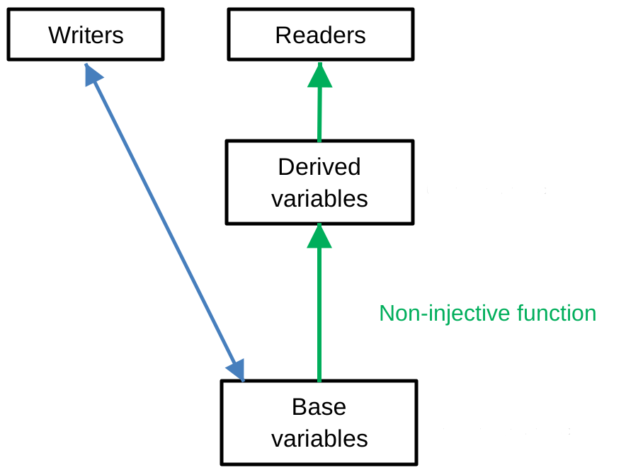
One of the great things about this approach is that it is optimal for writers, and allows for readers
to be fully asynchronous and to use a different schema, so we can optimise for readers as well.
An emphasis on immutable data makes it easier to merge concurrent edits - so
Operational Transformation is more efficient.
In a fully asynchronous distributed system (so there are no synchronised clocks), there is a natural
generalisation of time called a vector time,
and the states of the system that preserve causality form a lattice.
Vector times play an important role in event streaming in a fully asynchronous distributed system
(see multiple producers and consumers
which represents simple, efficient, reliable, exactly once "publish-subscribe" with multiple
publishers and multiple subscribers)
47 Database Trigger
A database trigger is procedural code that is automatically executed in response to
certain events such as inserts/deletes/updates on a particular base or derived relvar (i.e. a view)
in a database.
Note that allowing triggers on changes to views is very powerful. The views can be
non-injectve functions of the base representation (i.e. they can hide information). Views involve
the full power of the relational algebra to tranform the underlying base representation, providing
complete control over what information is visible to consumers of the information.
It's useful for applications/services to be able to define asynchronous triggers. Furthermore
this should allow for EOIO (exactly once in order) processing of the state changes.
The combination of database replication and database triggers provide a simpler alternative to
event messaging.
For a DBMS this represents a small overhead - the DBMS already deals with changes to the data -
for example it typically uses a log to represent changes to the data to implement atomicity and
recovery.
See how database triggers feature in the recommended approach to implementing long running business processes.
48 Asynchronous updates
In an atemporal relational database, there is a convention that the predicates don't
explicitly mention time, but rather refer implicitly to a single world situation at a single
moment in time.
To the extent that the relvars correctly record the extensions of their predicates about
the world, they should be synchronised with the world as it changes.
But of course, there are delays (inevitably because information cannot propagate faster than
the speed of light), and of course manual data entry by users involves delays.
In other words, the reality is normally that the information going into a database comes from asynchronous
sources, and the idea that the database records a synchronous snapshot of the world is a fiction.
It doesn't seem possible to make the predicates explicitly account for lags in the updates to
the relvars.
Nevertheless, at least for a database on a single machine, it is usual for transactions
to allow changes to multiple relvars to be made atomically, and therefore
it's usual for constraints to be imposed across relvars on the assumption that they are
updated synchronously.
But it's not a good idea to try to synchronise updates to multiple databases in a distributed
system.
Distributed transactions are an anti-pattern.
It seems necessary to treat the relvars that are not synchronised as belonging to
independent logical systems (microworlds).
This eliminates the logical contradictions because it is no longer assumed that the relvars record
conflicting information about the same world situation.
Presumably such contradictions tend to be short lived and are only an artifact of asynchronous
updates, and the conflicts should disappear at quiescence.
49 Compensating actions
When integrity constraints are imposed there is a tendency for update operations to become
more complex and fragile. Sometimes multiple changes must be made in a single atomic transaction
in order to satisfy the constraints.
One approach is to make complex update operations look easy by defining compensating actions.
These are additional implicit updates that are performed by an update operation. The idea is to make an
update more complex than it appears to be.
An example of a compensating action is a cascading delete:
a foreign key with cascade delete means that if a record in the parent table is deleted,
then the corresponding records in the child table will automatically be deleted.
Sometimes compensating actions are defined using triggered procedures. A triggered procedure cannot be called
explicitly, and instead executes automatically in response to events such as insertions, updates or deletions
on rows in a table.
A compensating action is also called a propagation constraint [].
The term propagation constraint seems unfortunate (one might hope the word constraint is reserved for the constraints
declared on the database value).
Also the term propagation constraint should not be confused with the term
transition constraint [] which means something else.
Also, the term compensating action should not be confused with a
compensating transaction [] which means something else.
It could be argued by the
Principle of least astonishment [] that it isn't reasonable for an update operation on one base variable to implicitly update another.
It seems better for update operations to have fixed semantics, rather than allow user-defined compensating
actions to be defined to modify their behaviour.
There is an alternative approach, which is generally superior, particularly when complex constraints
need to be imposed.
It is to instead impose constraints indirectly using non-injective
functions on the base variables.
Compensating actions tend to be laborious to define compared to using non-injective functions to impose constraints.
50 How to implement long running business processes
The following is a proposed approach for implementing long running business processes.
This approach isn't conventional - it shuns all application/service level IPC including event messaging
instead leaving all IPC up to the DBMS, where it's about data replication, not messaging.
It requires some capabilities of the DBMS and programming language(s) which are often
unavailable in current products on the market.
- Partition the business into parts (called services) which are somewhat independent.
Make sure these represent vertical slices - i.e. slices through the business domain.
For example Sales, Inventory, and Shipping services.
Note that horizontal slicing is an antipattern.
The vertical slices should separate concerns, and be:
- autonomous
- loosely coupled
- highly cohesive
- Assign software teams to vertical slices
- Use multidisciplinary software teams that encompass:
- requirements / design / implementation / testing
- documentation
- database schema / logic or function / UI
- Use a multi-master replicated embedded distributed DBMS to provide high performance, fault tolerance
and availability (such as CEDA).
Whereever possible applications/services only access data in their local database. This should be
automatically cached in memory by the DBMS.
- Use the relational model to record the current state of the business, typically using predicates
about business events that occur in the world, such as the receival of an order by the Sales
service.
- Don't impose constraints on base representations, instead impose constraints on read-only views
- Don't use Object Relational Mapping (ORM) to map tuples
in relations into object instances. ORM is an antipattern.
Instead use a language where typed relations and tuples are first class citizens.
- Only use a layered design within a process. For example, an application separates
data/function/UI within its process.
This is analogous to a three-tier design, but without deploying the layers to separate processes
or physical machines and using IPC between them.
- Wherever possible avoid IPC in application code.
This includes messaging between processes.
Don't use message brokers like RabbitMQ, NServiceBus or Kafka.
Message brokers represent an antipattern.
Only use in-process messaging (e.g. GUI event handlers or I/O completion events).
- Use views (which are usually read-only derived relvars maintained with incremental computing) for
logical independence to control what information
managed by one service is visible to others.
Note that logical independence provides loose coupling, information hiding and immunisation from
database schema changes.
- Use database triggers (typically defined on read-only derived relvars) to
process events as required.
- Be careful with defining appropriate atomic transactions on a local database.
A transaction should always "balance" in a manner which is analogous to
double entry bookkeeping [].
See
bank transfers without distributed transactions and
Making an on-line purchase.
For example removal of stock from an inventory account balances a commitment to ship that stock
to a customer.
The latter might trigger the shipping to be done by the Shipping service via a database trigger on a
derived relvar which is replicated on a remote machine.
51 Interfacing CEDA to a conventional RDBMS
CEDA has primarily been designed to support the writing of data.
It supports collaborative data entry by many users.
A conventional RDBMS is better suited to certain forms of read-only data processing,
e.g. adhoc queries, data mining, data reporting and presentation.
For that reason it is often appropriate to use a hybrid system.
CEDA is well suited to efficiently pushing data into an RDBMS.
This is straightforward because it is possible to process notifications of all changes to the
data in the database, whether from local or remote users.
Another consideration is the partitioning of the data (an important notion in CEDA).
It doesn't make sense to replicate all data everywhere, that doesn't scale.
52 Imperative programming language variables
The following is concerned with clarifying what is meant by
imperative programming language variables - i.e. variables which are
accessed by imperative statements in imperative programming languages, and not
to be confused with variables used in other contexts - such as variables
appearing in:
- set builder syntax
- formulas of first order logic
- logic programming languages
- functional programming languages
Chris Date in his book An Introduction to Database Systems characterises
a variable as follows:
A variable is a holder for an appearance of a value. A variable does
have a location in time and space. Also, of course, variables, unlike values,
can be updated; this is, the current value of the variable in question
can be replaced by another value, probably different from the previous one.
(Of course, the variable in question is still the same variable after the
update.)
Obviously, this is only informal and only intended to be used to
introduce the basic notions of values, variables and types. Nevertheless this
characterises a variable as what could more accurately be described as a mutable
L-value in a physical computer.
In the following, source code refers to a program text written in an imperative
programming language.
Read only variables
Chris Date's characterisation assumes a variable is updatable. That ignores the
important and very common notion of read-only variables. For example:
- Variables physically recorded in read only memory (ROM), read-only optical
media etc
- Dependent variables - i.e. variables which are derived (calculated) from
independent variables.
- Variables that only permit read-access for security reasons
Variables for abstract computational machines
A physical computational machine refers to a physical computer
that exists in space and time.
An abstract computational machine refers to a computational
machine defined in a pure mathematical formalism, which doesn't exist
physically in space and time.
Chris Date's characterisation speaks of variables existing in space and time
which apparently assumes that variables (only) exist on physical computers
For the purposes of defining a platform independent imperative programming
language, it is appropriate to define semantics in a pure mathematical
formalismn - i.e. for an abstract machine. Therefore any notion of programming
variables is defined in relation to an abstract machine. Any notions of some
correspondence to a physical machine is an implementational detail, and outside
the scope of the language specification.
Variables versus L-values
The following distinctions are made:
A L-value is a holder for the appearance of a value
within a computational machine - what perhaps might be called a storage location.
Whether the computational machine is abstract is unspecified, but as noted
above a language specification generally defines semantics on an abstract
machine, and in that case a L-value would be abstract we well.
It is possible to distinguish between read-only L-values and mutable
L-values.
A variable is an individual identifier appearing in source
code which is used to refer to an L-value.
An L-value expression is an expression appearing in source code
that denotes a L-value.
An R-value expression is an expression appearing in source code
that denotes a value.
The L-value / R-value distinction originated with Strachey 1963.
For example in the following C++ code, array is a variable, array[3] is an
L-value expression and i+j is an R-value expression. Note that the elements of
the array are L-values not variables.
int array[10];

array[3] = i+j;
Denotations on expressions
A common way to help define programming language semantics is to define denotations
on expressions that conform to a grammar. A denotation can be given for both
L-value expressions and R-value expressions.
In these terms, updating through a view is concerned with defining which RA
expressions are L-value expressions (not R-value expressions) and giving
denotations as L-values on them.
53 Conditionally existent L-values
One can speak of L-values being created and deleted over time.
L-value expressions sometimes denote a L-value and sometimes don't - i.e. whether
an expression denotes a L-value can change over time.
E.g. in C++
    std::vector<int> L;
    L[3] = 7;         // CRASH!!!, L[3] doesn't denote a L-value at this point in time
    L.resize(10);     // create 10 variables
    L[3] = 7;         // ok now L[3] denotes a L-value
It is useful to have a separation of concerns between
- expressions that denote L-values
- operations that efficiently update particular types of L-values (such as
an increment operation on an integer, or an append operation on a list).
E.g. in C++ modulo assignment is available on int variables so one might use
it on an element of L in a statement like this:
L[3] %= 10;
There is a separation of concerns between
- the expression L[3] that denotes an L-value; and
- the update operation using %=.
We want the same separation of concerns for updating a relational database, so we’re after
expressions that denote L-values that can be assigned any value of their type.
E.g. maybe something like this appends to a string attribute within a tuple
append( S WHERE S# = S#('S1') {CITY}, "x")
Prime factorisation of possreps doesn't (on its own) capture the most general
notion of separability that is sufficient for possrep components to be independently
updateable without risk of constraint violations.
For example, consider an implementation of an update operator, which contains a
lexical scope within which a reference to an L-value has been bound, perhaps
to a component of a tuple within a relvar. Within that lexical scope the reference
to the L-value can be passed to update operators that efficiently update the
L-value in-place. There are many such cases where the L-value can be assigned
any value of its type without risk of constraint violations.
The prime factor concept appears to be applicable to the special case where both
the existence and uniqueness of a specified binding to a pseudovariable that
supports infallible assignment is guaranteed. More generally a concept of
conditional binding is needed (such as when you want to bind a pseudovariable to
the eye colour of Fred Flintstone, but that is conditional on finding the
relevant tuple in the database in the first place).
It appears this idea of conditional existence of pseudovariables supporting
infallible assignment is related to updatable views. E.g. an updateable view
on Fred Flintstone's attributes. A user can be presented with this view and
update it as though it's a separate database - i.e. without surprises because
of integrity constraints depending on information that isn't visible in that
view. Also there are no update ambiguities. It's as though there's a "separable"
database nested within a containing database. The existence of the inner
database is conditional (and in fact the outer database is able to delete
the inner one).
54 Matches function to check whether the dbvar has a given dbvalue
In the following it is shown we can construct a relational algebra expression to test
whether the dbvar exactly matches a given dbvalue in schema `S`.
Given a relation `r` and a set of attributes `a`, let `π_a(r)` denote the projection of `r` onto `a`.
Note that `π_ϕ(r)` denotes the projection of r onto the empty set of attributes and
gives DUM if `r` is empty, otherwise DEE.
Given a relation `r`, let `empty(r) =` DEE`\\ π_ϕ(r)`.
This gives DEE if `r` is empty otherwise DUM.
Given union compatible relations `r` and `s`, let `r△s = (r\\s) ∪ (s\\r)` denote the
symmetric difference [].
Let `eq(r,s) = empty(r△s)`. This evaluates to DEE if r=s, otherwise DUM.
Let `d[R]` denote the value of relvar `R ∈ relvars(S)` in database value `d ∈ C(S)`.
Given database value `d ∈ C(S)`, let `matches(d) = ⋈ { eq(R,d[R]) | R ∈ relvars(S) }`
denote a relational algebra expression which evaluates to DEE if the dbvar
for schema `S` has value `d`, otherwise DUM.
Part VII: Examples and exploratory notes
This part collects examples and exploratory notes that illuminate the main
theory or suggest directions for further development.
55 Objects in two rooms example
Let there be two rooms. Let there be a predicate:
    p(OBJECT#, ROOM#) =
        object OBJECT# is in room ROOM#
Let B be a base relvar with attributes {OBJECT#, ROOM#} and there are views on B defined as
    V1 = RemoveDuplicates(B WHERE (ROOM# = 1), { OBJECT# })
    V2 = RemoveDuplicates(B WHERE (ROOM# = 2) , { OBJECT# })
    V3 = RemoveDuplicates(B, { OBJECT# })
Let a user of the database that is concerned with "what is supposed to be the case" according
to the database, with regarded to predicate p(OBJECT#, ROOM#) work on the assumption that the
extension of that predicate is given by V3.
Consider a change to the world situation where an object is moving from room 1 into room 2.
If the users update the database without delay then a tuple will be deleted from V1 as the
object exits room 1, and later a tuple is inserted into V2 as the object enters room 2.
In that case there are no duplicates in B and so B always equals V3.
Suppose instead that users issue updates with significant delays, and it so happens that the
insertion of a tuple into V2 is performed first.
Since B doesn't enforce a key constraint on OBJECT#, and the new tuple has a different
ROOM#, a distinct tuple is inserted into B.
The effect however is for a tuple to be deleted from V3 (because V3 strips away duplicates).
It is as though V3 carries an assumption that the world situation corresponds to the case of the
object still being in transit between the two rooms (or any other possible explanation).
Clearly this is arbitrary (and not even necessarily wrong - for all we know the object has just
exited room 2 and is on its way back again).
The important thing to note is that we already know that the database isn't being kept in sync
with the world situation (because of the delays in the updates which were assumed in order
for duplicates in B to be seen) so we have no right to claim the approach is illogical
according to "what is supposed to be the case".
Keep in mind that it is a given application requirement that a user performing data entry
is only authoritative for a single room.
The delays in applying updates are large enough that there are temporary inconsistencies.
This is regarded as an inevitable limitation in the sources of information used to update the
database, which is ironical given that the database is supposed to be recording consistent
snapshots of the world.
There isn't even an assumption that a user is providing updates for every change that actually
occurs in their room (e.g. while the user isn't looking an object exits and reenters the room).
In that case, according to the information available to the database it is never possible to
infer that particular world situations actually occur.
So any recorded world situation is an "artifact" - which is nevertheless useful to users not
bothered by the fact that it's a simplified approximation of the truth.
Possible solutions:
- Require users to be authoritative for both rooms, and to apply updates they really
do represent world situations that actually occur. But is this possible?
- Require users to make updates with less delay, so that temporary inconsistencies cannot
occur. But is this possible?
- Have the database reject updates that cause temporary inconsistencies.
This might annoy the hell out of them (because they may have to wait until an update succeeds).
Ironically this makes it even more likely that the database isn't up to date (and in
systems with more onerous integrity constraints, users may have to spend a lot more time
preparing complex changes in GUIs (e.g. using dialogs), that only update the database
when they click on the "apply" button or whatever.
This increases delays and aggravates the problems of asynchronous updates.
- Don't put the information from both rooms into the same database, so no-one can write a
query that assumes a consistent snapshot.
- Allow for inconsistencies, and calculate an "artifact" which is consistent across both
rooms (say by removing duplicates, or by giving precedence to one room over the other -
perhaps according to which update was performed most recently).
The 5th option seems best in practise.
56 Musings on the Relational Model
The Relational Model is of central importance to data management.
Relaxing constraints on the base relvars serves two purposes. It allows for concurrent data entry of relations
using Operational Transformation - mainly because it promotes
independently updatable variables,
and it addresses the view update problem which is considered in the context
of alternative representations (possreps) of the information recorded in the database.
Maximising orthogonality of information suggests the idea of nested relational databases.
Every non-empty relation has a unique prime Cartesian factorisation.
2011-09-15 Nested Data Models.docx is concerned with the question of a maximal partition of the information in a database into orthogonal parts. This means having as many
variables as possible which can be updated independently (with an emphasis on relvars and encompassing both base and derived relvars).
is concerned with the question of a maximal partition of the information in a database into orthogonal parts. This means having as many
variables as possible which can be updated independently (with an emphasis on relvars and encompassing both base and derived relvars).
2013-02-21 Type Systems.doc
concerns a formalism of some the ideas of Chris Date and Hugh Darwen expressed in The Third Manifesto, particularly their Inheritance Model
which could be described as subtype as subset and where the types form a lattice.
2013-11-15 Proposal for type system.doc
is another formalism of type systems.
Links